Mizer provides a range of plotting functions for visualising the results
of running a simulation, stored in a MizerSim object, or the initial state
stored in a MizerParams object.
Every plotting function exists in two versions, plotSomething and
plotlySomething. The plotly version is more interactive but not
suitable for inclusion in documents.
Details
This table shows the available plotting functions.
| Plot | Description |
plotBiomass | Plots the total biomass of each species through time. A time range to be plotted can be specified. The size range of the community can be specified in the same way as for getBiomass. |
plotSpectra | Plots the abundance (biomass or numbers) spectra of each species and the background community. It is possible to specify a minimum size which is useful for truncating the plot. |
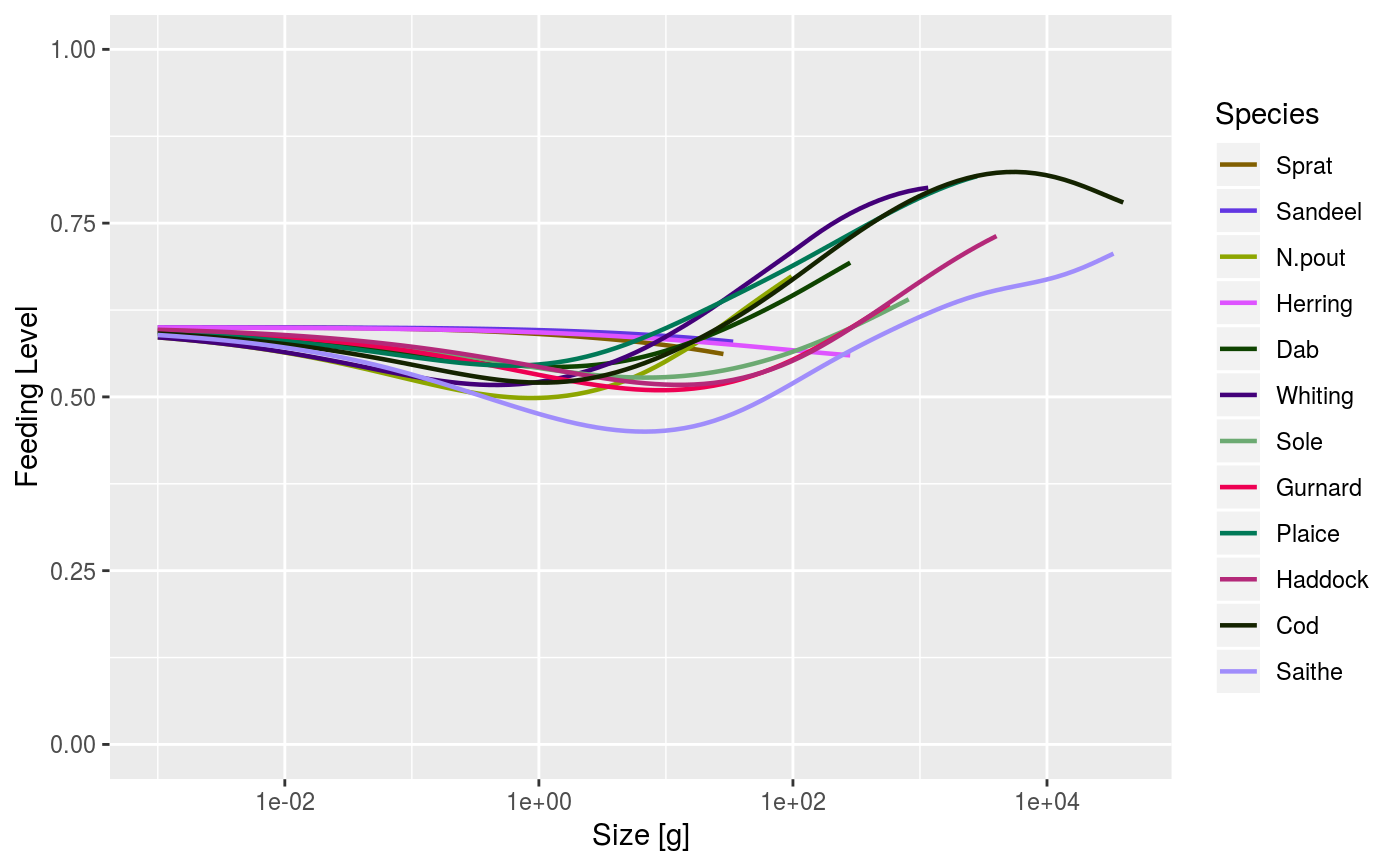
plotFeedingLevel | Plots the feeding level of each species against size. |
plotPredMort | Plots the predation mortality of each species against size. |
plotFMort | Plots the total fishing mortality of each species against size. |
plotYield | Plots the total yield of each species across all fishing gears against time. |
plotYieldGear | Plots the total yield of each species by gear against time. |
plot | Produces 5 plots (plotFeedingLevel, plotBiomass, plotPredMort, plotFMort and plotSpectra) in the same window as a summary. |
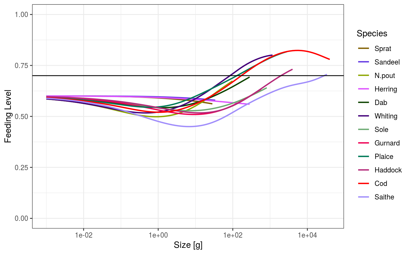
These functions use the ggplot2 package and return the plot as a ggplot
object. This means that you can manipulate the plot further after its
creation using the ggplot grammar of graphics. The corresponding function
names with plot replaced by plotly produce interactive plots
with the help of the plotly package.
While most plot functions take their data from a MizerSim object, some of those that make plots representing data at a single time can also take their data from the initial values in a MizerParams object.
Where plots show results for species, the line colour and line type for each
species are specified by the linecolour and linetype slots in
the MizerParams object. These were either taken from a default palette
hard-coded into emptyParams or they were specified by the user
in the species parameters dataframe used to set up the MizerParams object.
The linecolour and linetype slots hold named vectors, named by
the species. They can be overwritten by the user at any time.
Most plots allow the user to select to show only a subset of species,
specified as a vector in the species argument to the plot function.
The ordering of the species in the legend is the same as the ordering in the species parameter data frame.
Sometimes one wants to show two plots side-by-side with the same axes and
the same legend. This is made possible for some of the plots via the
displayFrames function.
See also
summary_functions, indicator_functions
Other plotting functions:
animateSpectra(),
displayFrames(),
plot,MizerSim,missing-method,
plotBiomass(),
plotDiet(),
plotFMort(),
plotFeedingLevel(),
plotGrowthCurves(),
plotPredMort(),
plotSpectra(),
plotYieldGear(),
plotYield(),
plotlyBiomass(),
plotlyFMort(),
plotlyFeedingLevel(),
plotlyGrowthCurves(),
plotlyPredMort(),
plotlySpectra(),
plotlyYieldGear(),
plotlyYield()
Examples
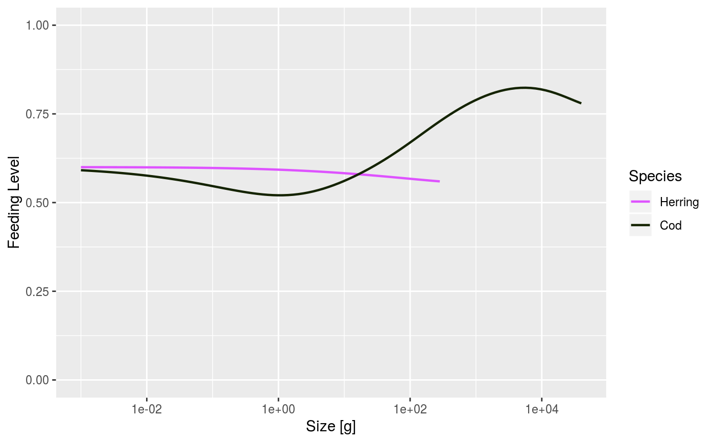
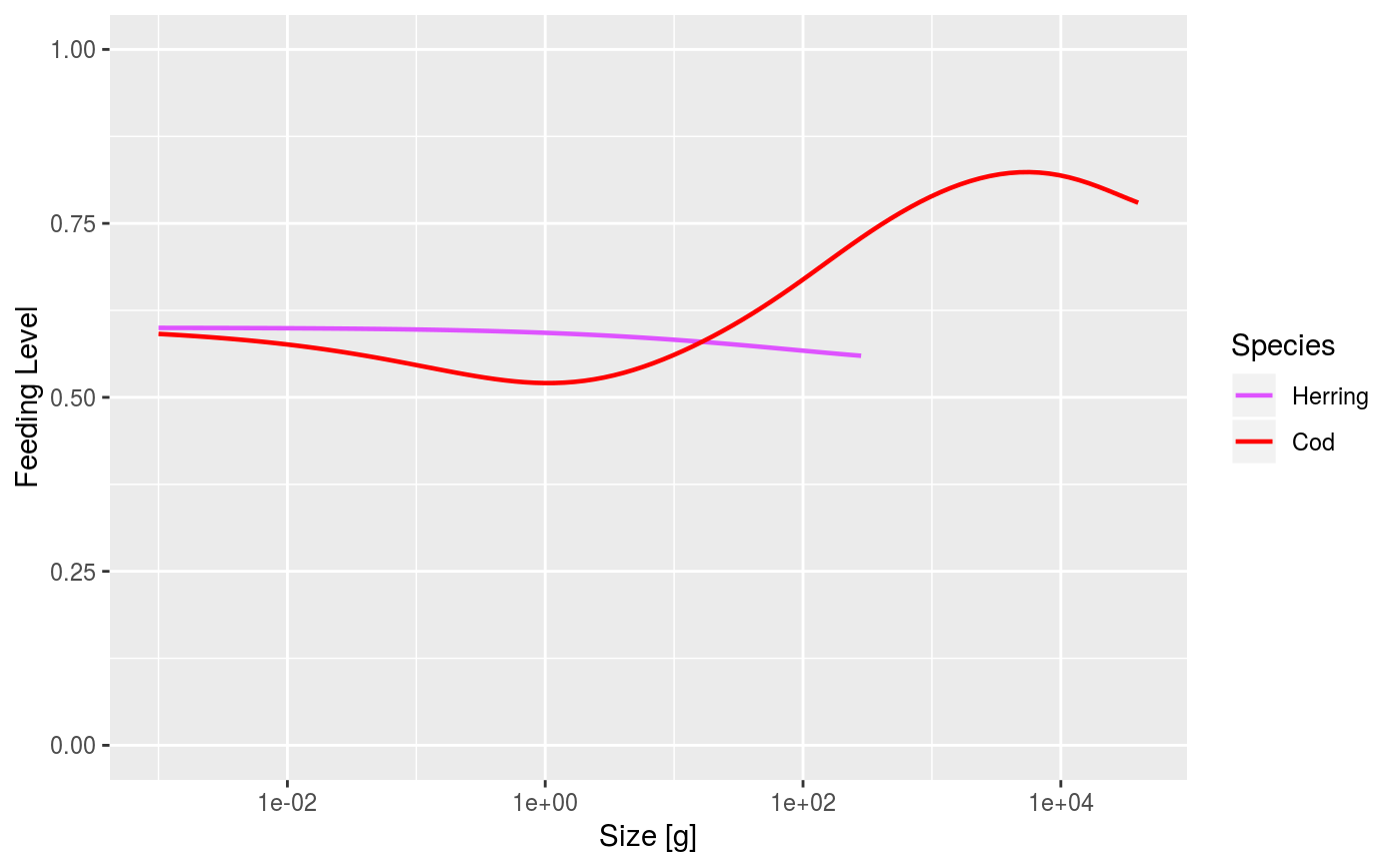
# Set up example MizerParams and MizerSim objects data(NS_species_params_gears) data(inter) params <- suppressMessages(newMultispeciesParams(NS_species_params_gears, inter)) sim <- project(params, effort=1, t_max=20, t_save = 2, progress_bar = FALSE) # Some example plots plotFeedingLevel(sim)# Specifying new colours and linetypes for some species sim@params@linetype["Cod"] <- "solid" sim@params@linecolour["Cod"] <- "red" plotFeedingLevel(sim, species = c("Cod", "Herring"))# Manipulating the plot library(ggplot2) p <- plotFeedingLevel(sim) p <- p + geom_hline(aes(yintercept = 0.7)) p <- p + theme_bw() p