9 Spatial models
Individuals live somewhere and they move. Fish swim in and out of a marine reserve, seeds are blown by the wind, infected foxes wander into new territories. To keep track of where individuals are, we replace the population number \(N(t)\) by a population density \(u(x,t)\), so that \(\int_a^bu(x,t)\,dx\) is the number of individuals between \(a\) and \(b\). The models become partial differential equations. This week we derive them and ask two questions: how large must a protected area be for a population to survive in it, and how can random movement create regular spatial patterns?
By the end of this week you should be able to:
- explain the link between random movement and diffusion;
- derive the reaction–diffusion equation from a conservation law and Fick’s law, and choose appropriate boundary conditions;
- find the critical domain size for population persistence by linearisation and separation of variables;
- derive the conditions for a Turing instability, explain the roles of activator and inhibitor, and apply the conditions to given models.
Open the week 9 notebook in Colab
9.1 Random movement and diffusion
- How did the mean squared distance of the random walkers grow with time? How did it depend on the step length \(\delta\) and the time \(\tau\) between steps?
- What relation between \(D\), \(\delta\) and \(\tau\) made the histogram match the solution of the diffusion equation?
- A fox moves a random 1 km every day. Roughly how far from home is it after 100 days? After a year?
You will be asked to relate random-walk parameters to diffusion coefficients and to estimate typical distances travelled.
A walker making independent steps \(\pm\delta\) every time \(\tau\) has, after \(n=t/\tau\) steps, mean position \(0\) and mean squared displacement \(n\delta^2=2Dt\) with \[ D=\frac{\delta^2}{2\tau}. \] The typical distance grows like \(\sqrt t\), not like \(t\). The density of many walkers is described by the diffusion equation \(\partial_tu=D\partial_x^2u\), whose solution starting from a point is the Gaussian \(u=\frac{1}{\sqrt{4\pi Dt}}e^{-x^2/(4Dt)}\). For the fox, \(D=0.5\) km²/day: after 100 days it is typically about 10 km from home, after a year about 19 km.
9.2 The reaction–diffusion equation
Let the flux \(J(x,t)\) be the net number of individuals crossing the point \(x\) from left to right per unit time, and let \(f(u)\) be the local net growth rate (births minus deaths per unit length).
- Explain why, for any interval \([x_0,x_0+\Delta x]\), \[\frac{\partial}{\partial t}\int_{x_0}^{x_0+\Delta x}u\,dx=\int_{x_0}^{x_0+\Delta x}f(u)\,dx+J(x_0)-J(x_0+\Delta x).\]
- Divide by \(\Delta x\) and let \(\Delta x\to0\) to get \(\partial_tu=f(u)-\partial_xJ\).
- For random movement, more individuals move from crowded to less crowded places. Fick’s law says \(J=-D\,\partial_xu\). Explain the minus sign and derive the reaction–diffusion equation \[\partial_tu=f(u)+D\,\partial_x^2u. \tag{9.1}\]
- What is the flux at a boundary that no individual crosses? Write this as a condition on \(u\). What is the condition at a boundary beyond which every individual is immediately killed?
Part B solves the diffusion equation on an interval with either kind of boundary condition.
- With no-flux boundaries, what happens to the total population? What is the long-term state?
- With zero-population (“absorbing”) boundaries, what happens? How does the long-term shape of \(u\) look?
You will be asked to write down reaction–diffusion equations for described situations and to choose boundary conditions.
Conservation gives \(\partial_tu=f(u,x)-\partial_xJ\). For random motion \(J=-D\partial_xu\), since the net flow is down the density gradient, and hence \[ \partial_tu=f(u)+D\partial_x^2u. \] Boundary conditions:
- no flux (Neumann): \(\partial_xu=0\), e.g. a shoreline or a closed box;
- absorbing (Dirichlet): \(u=0\), e.g. the edge of a reserve beyond which everything is caught.
Diffusion alone smooths out differences. With no-flux boundaries it conserves the total and approaches a uniform state. With absorbing boundaries the population drains away. The interesting phenomena arise from the combination of reaction and diffusion.
9.3 How large must a reserve be?
A marine protected area extends from the shore at \(x=0\) to \(x=L\). Inside, fish grow logistically, are caught at a moderate rate \(E<r\), and move randomly. Outside the reserve fishing is so intense that every fish that leaves is caught, so \(u(L,t)=0\). At the shore there is no flux, so \(\partial_xu(0,t)=0\): \[ \partial_tu=ru\left(1-\frac uK\right)-Eu+D\partial_x^2u. \tag{9.2}\]
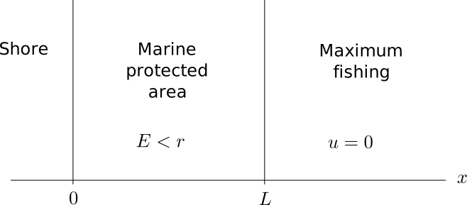
Without movement, the fish would persist whenever \(E<r\). With movement, fish are lost across \(x=L\). Will a small reserve still be enough? What should the critical width depend on?
- For \(r=1\), \(E=0.5\) and \(D=1\), find the critical width \(L_c\) below which the population dies out, to two significant figures.
- How does \(L_c\) change when you double \(D\)? When you change \(r-E\)? Guess a formula.
- Above \(L_c\), what does the population profile look like?
- Near extinction \(u\) is small. Linearise Eq. 9.2 about \(u=0\).
- Substitute \(u=X(x)T(t)\) and separate variables with separation constant \(\gamma\). Show that \(T=T(0)e^{\gamma t}\) and \(X''=-\rho^2X\) with \(\rho^2=(r-E-\gamma)/D\).
- Impose the boundary conditions to show \(X=A\cos(\rho x)\) with \(\rho_n=\frac{(2n+1)\pi}{2L}\), and \(\gamma_n=r-E-D\rho_n^2\).
- The population persists if the extinction state is unstable, i.e. if some \(\gamma_n>0\). Show that this happens iff \[L>L_c=\frac\pi2\sqrt{\frac{D}{r-E}}.\] Compare with your numerical result.
A proposed reserve would have width \(L=5\) km. The fish have \(r=0.8\) per year and \(D=2\) km²/year.
- What is the maximal fishing rate \(E\) inside the reserve that still allows the population to persist?
- Sketch the trade-off curve between \(L\) and the maximal allowed \(E\). Mark the region where the population persists.
- What are the most important limitations of this model?
You will be asked to find critical domain sizes and allowed harvesting rates for reaction–diffusion models with various boundary conditions.
The linearised equation \(\partial_tu=(r-E)u+D\partial_x^2u\) has separable solutions \(u_n=A_ne^{\gamma_nt}\cos(\rho_nx)\) with \(\rho_n=(2n+1)\pi/(2L)\) and \(\gamma_n=r-E-D\rho_n^2\). The general solution is a sum of these. The largest growth rate is \(\gamma_0\), so the population persists iff \(\gamma_0>0\): \[ L>\frac\pi2\sqrt{\frac D{r-E}}\qquad\Longleftrightarrow\qquad E<r-\frac{D\pi^2}{4L^2}. \] Losses across the boundary act like extra mortality \(D\pi^2/(4L^2)\), which is large for small reserves. The length scale \(\sqrt{D/(r-E)}\) is how far a fish typically moves during one “generation” \(1/(r-E)\). For \(r=1\), \(E=0.5\), \(D=1\) the critical width is \(L_c=\frac\pi2\sqrt2\approx2.22\). In the group task, \(E_{\max}=0.8-2\pi^2/100\approx0.60\) per year.
9.4 Patterns from diffusion: Turing instabilities
How do the spots of a leopard, the stripes of a zebrafish, or the regular patches of vegetation in semi-arid landscapes arise? In 1952 Alan Turing proposed a surprising mechanism: two interacting species that diffuse at different rates can turn a uniform state into a regular pattern, even though diffusion on its own smooths things out.
Consider two species with densities \(u\) and \(v\): \[ \partial_tu=f(u,v)+D_1\partial_x^2u,\qquad \partial_tv=g(u,v)+D_2\partial_x^2v. \tag{9.3}\] We use the example \[ f(u,v)=-u+u^2v,\qquad g(u,v)=b-u^2v, \tag{9.4}\] which has the uniform steady state \((u^*,v^*)=(b,1/b)\).
Part D starts from the uniform state plus a tiny random perturbation. It shows \(u(x,t)\) as a coloured space–time picture and the final profile.
- Take \(b=1.5\) and \(D_1=1\). Without diffusion (in the notebook, the local dynamics alone), is \((b,1/b)\) stable?
- Increase \(d=D_2/D_1\) from \(1\). For which values does a pattern appear? Find the threshold roughly.
- How does the wavelength (the distance between peaks) depend on \(d\)? Does it depend on the domain length \(L\)?
- Which species must diffuse faster?
Linearise about \((u^*,v^*)\): \(u=u^*+\xi\), \(v=v^*+\eta\), and let \(a_{ij}\) be the entries of the Jacobian \(A\) of \((f,g)\) at the steady state.
- Try \(\xi=B_1e^{\sigma t}\cos(kx)\) and \(\eta=B_2e^{\sigma t}\cos(kx)\). Show that \(\sigma\) must be an eigenvalue of \[A(k)=\begin{pmatrix}a_{11}-D_1k^2&a_{12}\\a_{21}&a_{22}-D_2k^2\end{pmatrix}.\]
- Assume the steady state is stable without diffusion (\(\operatorname{tr}A<0\), \(\det A>0\)). Show that \(\operatorname{tr}A(k)<0\) for all \(k\).
- Show that \(\det A(k)=D_1D_2k^4-(D_1a_{22}+D_2a_{11})k^2+\det A\). Explain why an instability requires this quadratic in \(k^2\) to become negative for some \(k^2>0\), and derive the conditions \[D_1a_{22}+D_2a_{11}>0,\qquad (D_1a_{22}+D_2a_{11})^2>4D_1D_2\det A.\]
- Show that these conditions, together with \(\operatorname{tr}A<0\), force \(a_{11}\) and \(a_{22}\) to have opposite signs and require \(D_1\neq D_2\).
For the model Eq. 9.4:
- Compute the Jacobian at \((b,1/b)\). Which species is the activator (it promotes its own growth, \(a_{ii}>0\)) and which is the inhibitor?
- Check the four conditions and show that a Turing instability requires \(b>1\) and \(d=D_2/D_1>b^2(3+\sqrt8)\). Compare with the threshold you found for \(b=1.5\).
- On the finite domain \([0,L]\) with no-flux boundaries, the allowed wave numbers are \(k_n=n\pi/L\). Why? What does this imply for small domains?
You will be asked to compute Jacobians of reaction–diffusion models at uniform steady states, check the Turing conditions and find threshold diffusion ratios.
A uniform steady state that is stable without diffusion is driven unstable by diffusion iff \[ \begin{aligned} &\text{(a) } a_{11}+a_{22}<0, &&\text{(b) } a_{11}a_{22}-a_{12}a_{21}>0,\\ &\text{(c) } D_1a_{22}+D_2a_{11}>0, &&\text{(d) } (D_1a_{22}+D_2a_{11})^2>4D_1D_2(a_{11}a_{22}-a_{12}a_{21}). \end{aligned} \] Conditions (a) and (b) are stability without diffusion. Conditions (c) and (d) make \(\det A(k)<0\) on an interval \(k_-<k<k_+\) with \[ k_\pm^2=\frac{D_1a_{22}+D_2a_{11}\pm\sqrt{(D_1a_{22}+D_2a_{11})^2-4D_1D_2\det A}}{2D_1D_2}. \] Perturbations with these wave numbers grow, giving a pattern with wavelength about \(2\pi/k\), set by the parameters rather than the domain. One species must be an activator (\(a_{11}>0\), say) and the other an inhibitor (\(a_{22}<0\)), and the sign pattern of \(A\) must be \(\begin{pmatrix}+&-\\+&-\end{pmatrix}\) or \(\begin{pmatrix}+&+\\-&-\end{pmatrix}\). From (a) and (c), \(D_1/D_2<-a_{11}/a_{22}<1\): the inhibitor must diffuse faster than the activator (“local activation, long-range inhibition”).
For the example, \(A=\begin{pmatrix}1&b^2\\-2&-b^2\end{pmatrix}\), so \(u\) is the activator and \(v\) the inhibitor. The conditions give \(b>1\) and \(d>b^2(3+\sqrt8)\approx5.83b^2\), i.e. \(d>13.1\) for \(b=1.5\). On \([0,L]\) with no-flux boundaries only \(k_n=n\pi/L\) are allowed, so a pattern needs \(\pi/L<k_+\): small domains stay uniform.
Individuals may also move towards higher concentrations of a chemical (chemotaxis), with flux \(J=\chi n\,\partial_xa\). Slime mould amoebae secrete an attractant \(a\) themselves. With production rate \(h\) and decay rate \(q\): \[ \partial_tn=-\chi\partial_x(n\partial_xa)+D_n\partial_x^2n,\qquad \partial_ta=hn-qa+D_a\partial_x^2a. \] Linearising about the uniform state (\(hn^*=qa^*\)) with modes \(\cos(kx)\) gives \[ A(k)=\begin{pmatrix}-D_nk^2&\chi n^*k^2\\h&-q-D_ak^2\end{pmatrix},\qquad \det A(k)=D_nD_ak^4+(D_nq-h\chi n^*)k^2. \] The trace is always negative, but the determinant is negative for small \(k\) if \(h\chi n^*>D_nq\): the amoebae aggregate if they produce enough attractant and do not diffuse too fast. On \([0,L]\) with no-flux boundaries this requires in addition \(L>\pi\sqrt{D_nD_a/(h\chi n^*-D_nq)}\).
9.5 Exam-style questions
Fish in a river of width \(L\) satisfy \[ \frac{\partial F}{\partial t}=rF\left(1-\frac FK\right)+D\frac{\partial^2F}{\partial x^2},\qquad 0<x<L, \] with positive constants \(r,K,D\). There is no flux at \(x=L\), while fishermen on the bank at \(x=0\) catch every fish that gets there, so \(F(0,t)=0\).
Find the spatially uniform steady states of the PDE without boundary conditions and indicate their stability. [2 marks]
Linearise the equation for small \(F\). [1 mark]
With \(F=e^{\lambda t}(A\cos kx+B\sin kx)\) show that \(\lambda_n=r-k_n^2D\) with \(k_n=(2n+1)\pi/(2L)\). [5 marks]
Hence find the minimum width of the river for the population to persist. [2 marks]
\(F=0\) (unstable, since \(r>0\)) and \(F=K\) (stable).
\(\partial_tF=rF+D\partial_x^2F\).
Substituting: \(\lambda=r-Dk^2\). \(F(0,t)=0\) gives \(A=0\). \(\partial_xF(L,t)=0\) gives \(Bk\cos(kL)=0\), so \(kL=(2n+1)\pi/2\).
Persistence requires \(\lambda_0>0\): \(r>D\pi^2/(4L^2)\), i.e. \(L>\frac\pi2\sqrt{D/r}\).
Consider \[ \partial_tu=a-u+u^2v+D_1\partial_x^2u,\qquad \partial_tv=b-u^2v+D_2\partial_x^2v, \] with \(b>0\) and \(a+b>0\). Show that the uniform steady state is \((u^*,v^*)=(a+b,\,b/(a+b)^2)\) and that it is driven unstable by diffusion iff \[ b-a<(a+b)^3,\qquad D_2\frac{b-a}{a+b}-D_1(a+b)^2>0,\qquad \left[D_2\frac{b-a}{a+b}-D_1(a+b)^2\right]^2>4D_1D_2(a+b)^2. \] [10 marks]
Adding \(f+g=a+b-u=0\) gives \(u^*=a+b\), and then \(g=0\) gives \(v^*=b/(a+b)^2\). The Jacobian entries are \(a_{11}=-1+2u^*v^*=\frac{b-a}{a+b}\), \(a_{12}=u^{*2}=(a+b)^2\), \(a_{21}=-2u^*v^*=-\frac{2b}{a+b}\) and \(a_{22}=-(a+b)^2\). Then \(\operatorname{tr}A<0\iff\frac{b-a}{a+b}<(a+b)^2\iff b-a<(a+b)^3\) (as \(a+b>0\)), and \(\det A=-(b-a)(a+b)+2b(a+b)=(a+b)^2>0\) always. Conditions (c) and (d) give the other two inequalities, since \(D_1a_{22}+D_2a_{11}=D_2\frac{b-a}{a+b}-D_1(a+b)^2\).
Consider \[ \partial_tc_1=\delta-kc_1-c_1c_2^2+D_1\partial_x^2c_1,\qquad \partial_tc_2=kc_1+c_1c_2^2-c_2+D_2\partial_x^2c_2, \] with \(k,\delta>0\). Find the uniform steady state and the conditions for it to be driven unstable by diffusion. Which species is the activator? [10 marks]
Adding the equations: \(\delta-c_2=0\), so \(c_2^*=\delta\) and then \(c_1^*=\delta/(k+\delta^2)\). The Jacobian is \[A=\begin{pmatrix}-(k+\delta^2)&-\frac{2\delta^2}{k+\delta^2}\\ k+\delta^2&\frac{\delta^2-k}{k+\delta^2}\end{pmatrix}.\] \(\det A=-(\delta^2-k)+2\delta^2=\delta^2+k>0\) always. The conditions are:
- \(\frac{\delta^2-k}{k+\delta^2}<k+\delta^2\);
- \(D_1\frac{\delta^2-k}{k+\delta^2}-D_2(k+\delta^2)>0\);
- \(\left(D_1\frac{\delta^2-k}{k+\delta^2}-D_2(k+\delta^2)\right)^2>4D_1D_2(k+\delta^2)\).
Condition (c) needs \(a_{22}>0\), i.e. \(\delta^2>k\). Then \(c_2\) is the activator, \(c_1\) the inhibitor, and \(c_1\) must diffuse faster: \(D_1/D_2>(k+\delta^2)^2/(\delta^2-k)>1\).
Summary
- Random walks with steps \(\delta\) every \(\tau\) lead to diffusion with \(D=\delta^2/(2\tau)\). Typical distances grow like \(\sqrt{2Dt}\).
- Reaction–diffusion: \(\partial_tu=f(u)+D\partial_x^2u\), from conservation and Fick’s law \(J=-D\partial_xu\). Boundaries are no-flux (\(\partial_xu=0\)) or absorbing (\(u=0\)).
- Critical domain size: linearise about \(u=0\) and separate variables. A reserve must be wider than \(\frac\pi2\sqrt{D/(r-E)}\).
- Turing instability: \(\det A(k)<0\) for a band of wave numbers. This needs an activator–inhibitor pair with the inhibitor diffusing faster.
9.6 Launch: invasion waves
Open the week 10 notebook in Colab
The grey squirrel was introduced to Britain around 1890 and spread steadily across the country. Muskrats released near Prague in 1905 spread across Europe with a front that advanced by a roughly constant distance each year.
- In part A, a population with logistic growth and diffusion, \(\partial_tu=ru(1-u)+D\partial_x^2u\), starts in a small region. Predict: how will the population spread? Will it speed up, slow down, or advance at a constant speed?
- Measure the speed of the front (the notebook fits it for you) for several values of \(r\) and \(D\). Make a table and guess a formula for the speed.
- In part B, the “population” is instead a disease spreading among foxes, where only the infected foxes move. Describe the wave. What is left behind the wave?
- Bring your table and conjectures to the first session of week 10.