1 Single-species models in continuous time
Population dynamics studies how the number of individuals in a population changes over time. The population could be the bacteria in a Petri dish, the deer in a forest, the cod in the Baltic Sea or the people in a country. We describe it by a function \(N(t)\) giving the number of individuals at time \(t\), with some initial value \(N(0)=N_0\). This week we ask a simple question: what can we say about \(N(t)\) if we know how the rate of change of \(N\) depends on \(N\) itself? The answer turns out to be “almost everything”, and without having to solve any differential equation.
TipLearning outcomes for this week
By the end of this week you should be able to:
- write down a differential equation for a population from assumptions about births, deaths, immigration and emigration;
- solve the exponential model and the exponential model with immigration;
- sketch solutions of \(dN/dt=f(N)\) from a graph of \(f\);
- find steady states and determine their stability both graphically and by linearisation;
- explain the logistic model and the (strong and weak) Allee effect, and interpret their parameters.
Open the week 1 notebook in Colab
1.1 Births, deaths and exponential growth
Four processes change the size of a population: births, deaths, immigration and emigration. So \[ \frac{dN}{dt} = \text{birth rate} - \text{death rate} + \text{immigration rate} - \text{emigration rate}. \tag{1.1}\] Here “rate” means number of individuals per unit time. A model is a statement about how these rates depend on \(N\) (and perhaps on other things).
NotePredict
A population of 1000 bacteria has a per-capita birth rate of \(b=0.3\) per hour and a per-capita death rate of \(d=0.1\) per hour, so that the population’s total birth rate is \(bN\) and its total death rate is \(dN\). Roughly how long will it take for the population to double? Write down your guess.
TipExplore: notebook part A
Run the setup cell and then the cell in part A. It solves \[ \frac{dN}{dt}=bN-dN \] and plots \(N(t)\) both on an ordinary scale and on a logarithmic scale.
- Find the doubling time for \(b=0.3\), \(d=0.1\). How good was your guess?
- Change \(b\) and \(d\) keeping \(b-d\) fixed. What do you notice?
- What does the graph of \(\log N(t)\) look like? What is its slope?
- What happens when \(b<d\)?
NoteExplain
- Write \(r=b-d\). Solve \(dN/dt=rN\) with \(N(0)=N_0\).
- Use your solution to show that the doubling time is \(t_d = \ln 2 / r\). Check this against your observation.
- Why does only the difference \(b-d\) matter? Why is the graph of \(\log N\) a straight line?
The exponential model is the oldest population model. It was proposed by Thomas Malthus in 1798. Notice that \(N(t)\) in this model takes non-integer values. For large populations this is harmless. For small populations the random timing of individual births and deaths matters and one would need a stochastic model. In this module all our models are deterministic.
WarningGroup task: immigration
A country currently has \(N_0=70\) million inhabitants. The per-capita death rate is \(d=0.015\) per year and the per-capita birth rate is \(b=0.01\) per year. In addition, \(a=300\,000\) people immigrate each year.
- Write down the ODE for \(N(t)\), using symbols rather than numbers.
- Before solving it: is there a population size at which the population stays constant? Will the population grow or shrink from its present size?
- Solve the ODE. (Hint: shift the dependent variable, \(M=N-N^*\), to turn it into the exponential model.)
- What is the projected population after 10 years? Check your answer with the immigration slider in part A of the notebook.
NoteCheck: feedback quiz 1.1
You will be asked to write down and solve linear population models from verbal descriptions and to compute doubling or halving times.
NoteConsolidation: exponential growth
If the per-capita birth rate \(b\) and death rate \(d\) are constants, then \[ \frac{dN}{dt} = (b-d)N = rN, \qquad N(t) = N_0 e^{rt}. \tag{1.2}\] The population grows exponentially if \(r>0\) and decays exponentially if \(r<0\). The doubling time (or halving time for \(r<0\)) is \(\ln 2/|r|\). The quantity \(r\) is a rate with units of 1/time. On a logarithmic scale the solution is a straight line with slope \(r\).
With constant immigration at rate \(a\): \[ \frac{dN}{dt}=rN+a, \qquad N(t) = N^* + (N_0-N^*)e^{rt}, \qquad N^*=-\frac{a}{r}. \] For \(r<0\) the population approaches the steady state \(N^* = a/(d-b)\). For the country above, \(N^*=60\) million and \(N(10)=60+10e^{-0.05}\approx 69.5\) million.
1.2 Limits to growth: the logistic model
No population can grow exponentially for ever. As it gets larger, food and space become scarce and the per-capita growth rate drops. The simplest assumption is that the per-capita growth rate decreases linearly with \(N\) and becomes zero at some population size \(K\): \[ \frac{1}{N}\frac{dN}{dt} = r\left(1-\frac{N}{K}\right) \quad\Longleftrightarrow\quad \frac{dN}{dt}=rN\left(1-\frac{N}{K}\right). \tag{1.3}\] This is the logistic model. \(K\) is called the carrying capacity.
NotePredict
Sketch, without any calculation, what you think \(N(t)\) looks like for the logistic model when (a) \(N_0\) is much smaller than \(K\), (b) \(N_0\) is a bit smaller than \(K\), and (c) \(N_0\) is larger than \(K\).
TipExplore: notebook part B
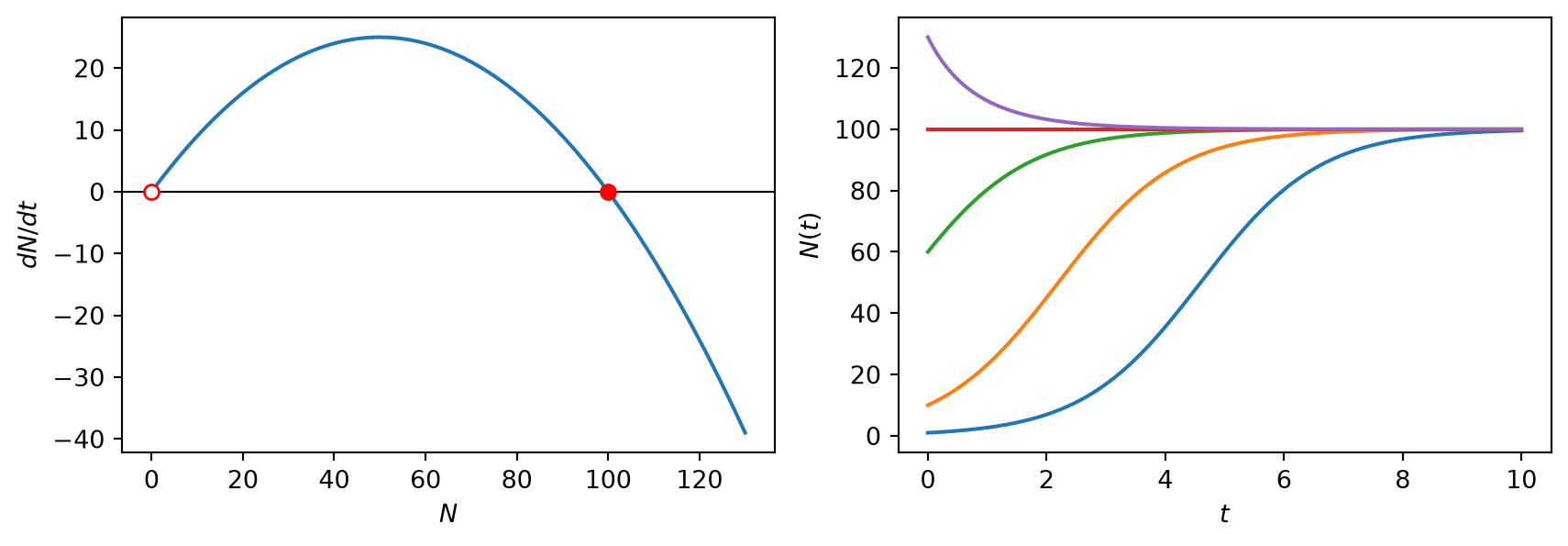
Part B shows two plots side by side: on the left the rate of change \(dN/dt\) as a function of \(N\), on the right solutions \(N(t)\) for several initial values.
- Compare the solutions with your sketches.
- At which population size is the population growing fastest? Find this on both plots. What feature of the left plot corresponds to the inflection point of the curves on the right?
- The red dots on the left plot mark values of \(N\) where \(dN/dt=0\). What do the solutions do near each of them?
- Can a solution ever overshoot \(K\) and then come back down? Can a solution oscillate? Try hard to make it happen.
NoteExplain
- The graph of \(f(N)=rN(1-N/K)\) is a parabola. Where does it cross the \(N\) axis? Where is its maximum and what is the maximum value?
- The slope of the graph of \(N(t)\) at time \(t\) equals \(f(N(t))\). Use this to explain why solutions starting in \((0,K)\) increase and those starting above \(K\) decrease, and why they get flatter as they approach \(K\).
- For \(dN/dt=f(N)\) with \(f\) continuously differentiable, solutions exist and are unique (Picard–Lindelöf). Use uniqueness to argue that a solution can never cross a steady state, and hence that solutions are monotonic: they can never oscillate.
The logistic equation can also be solved exactly (exam-style question 1.3): \[ N(t)=\frac{N_0 K e^{rt}}{K+N_0(e^{rt}-1)}. \tag{1.4}\] But the qualitative understanding you just gained is more useful. It works for any \(f\), including those for which the ODE cannot be solved.
NoteCheck: feedback quiz 1.2
You will be asked to find steady states from a formula for \(f(N)\), to identify the population size of maximal growth, and to match graphs of \(f(N)\) to graphs of solutions \(N(t)\).
NoteConsolidation: reading solutions off the graph of \(f\)
For an autonomous ODE \(dN/dt=f(N)\):
- Steady states are the zeros \(N^*\) of \(f\).
- Where \(f(N)>0\) solutions increase, where \(f(N)<0\) they decrease. We mark this with arrows on the \(N\) axis. This picture is the phase line.
- Solutions cannot cross steady states, so they are monotonic and approach a steady state (or \(\pm\infty\)) as \(t\to\infty\).
- \(N(t)\) has an inflection point exactly where \(f\) has a maximum or minimum, because \(\ddot N = f'(N)\dot N\).
For the logistic model, \(N^*=0\) and \(N^*=K\) are the steady states, the growth rate \(dN/dt\) is largest at \(N=K/2\) where it equals \(rK/4\), and all solutions with \(N_0>0\) approach \(K\).
1.3 Stability of steady states
A steady state is stable if solutions that start close to it stay close to it and approach it, and unstable if solutions that start close to it move away. In the logistic model \(N^*=K\) is stable and \(N^*=0\) is unstable. We now want a quick way to decide stability without drawing the whole graph.
TipExplore: notebook part C
Part C lets you type in any function \(f(N)\). For each steady state the notebook prints the slope \(f'(N^*)\). Try, for example, \[ f(N) = N(N-1)(3-N), \qquad f(N)=\sin(N), \qquad f(N)= N^2(2-N). \] Make a table with one row per steady state, listing the value of \(f'(N^*)\) and whether the steady state is stable or unstable (look at the solutions!). Formulate a conjecture. Is there a case your conjecture does not decide?
NoteExplain: linearisation
Write \(N(t)=N^*+n(t)\) with \(n\) small.
- Taylor expand \(f(N^*+n)\) to first order and show that \(\dfrac{dn}{dt}\approx f'(N^*)\,n\).
- Solve this linear equation and hence explain your conjecture.
- For \(f(N)=N^2(2-N)\) the steady state \(N^*=0\) has \(f'(0)=0\). What does the phase line tell you about its stability? (Such a steady state is called semi-stable.)
WarningGroup task
Each person in the group invents a function \(f(N)\) with at least three steady states in \(N\geq 0\) and draws the phase line. Swap with a neighbour, who sketches the solutions \(N(t)\) for several initial conditions and classifies the steady states by linearisation. Check each other’s work, and check with the notebook.
NoteCheck: feedback quiz 1.3
You will be asked to compute \(f'(N^*)\) at the steady states of a given model and to classify them as stable or unstable.
NoteConsolidation: linear stability analysis
Near a steady state \(N^*\) the perturbation \(n(t)=N(t)-N^*\) satisfies \[ \frac{dn}{dt}\approx f'(N^*)\,n \qquad\Longrightarrow\qquad n(t)\approx n(0)e^{f'(N^*)t}. \tag{1.5}\]
- If \(f'(N^*)<0\) the steady state is stable.
- If \(f'(N^*)>0\) the steady state is unstable.
- If \(f'(N^*)=0\) linearisation cannot decide. Look at the phase line or at higher-order terms.
The number \(1/|f'(N^*)|\) is the characteristic time scale of the approach to (or departure from) the steady state. For the logistic model \(f'(N)=r(1-2N/K)\), so \(f'(0)=r>0\) and \(f'(K)=-r<0\).
For more on one-dimensional dynamics see the first chapters of (Strogatz 2000).
1.4 The Allee effect
In the logistic model the per-capita growth rate is largest when the population is smallest. For many species this is wrong. W. C. Allee observed that at low densities individuals can do worse:
- flowers in sparse populations are visited less often by pollinators;
- wolves hunt more successfully in packs;
- colonial seabirds such as puffins rely on large colonies for protection;
- broadcast spawners such as sea urchins need a high density for fertilisation;
- small populations suffer from inbreeding.
An increase of the per-capita growth rate with \(N\) at low densities is called an Allee effect.
NotePredict
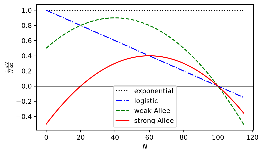
Sketch a graph of the per-capita growth rate \(\frac{1}{N}\frac{dN}{dt}\) against \(N\) for (a) exponential growth, (b) logistic growth, (c) a population with an Allee effect. What could make the difference between a “weak” and a “strong” Allee effect?
TipExplore: notebook part D
Part D explores the model \[ \frac{dN}{dt}=rN\left(1-\frac{N}{K}\right)\left(\frac{N}{K_0}-1\right). \tag{1.6}\] It shows the per-capita growth rate, the growth rate and solutions.
- Take \(0<K_0<K\). Describe what happens to populations starting below \(K_0\) and above \(K_0\).
- What is the ecological meaning of \(K_0\)?
- Now make \(K_0\) negative. How does the per-capita rate change? What happens to small populations now?
NoteExplain
- For \(0<K_0<K\), find the steady states of Eq. 1.6, determine their stability from the sign pattern of \(f\) and confirm this by linearisation.
- Explain why a strong Allee effect matters for conservation and for fisheries management.
NoteCheck: feedback quiz 1.4
You will be asked to classify the steady states of Allee-type models and to identify the threshold population size.
NoteConsolidation: weak and strong Allee effect
With a weak Allee effect the per-capita growth rate increases with \(N\) at low densities but stays positive. With a strong Allee effect it is negative for small \(N\). In model Eq. 1.6 with \(0<K_0<K\) the steady states are \(0\) (stable), \(K_0\) (unstable) and \(K\) (stable). Populations below the threshold \(K_0\) go extinct and populations above it approach \(K\). This threshold phenomenon is called critical depensation. It makes small populations extremely vulnerable, and we will meet it again when we study harvesting. For \(K_0<0\) the model has a weak Allee effect and \(0\) is unstable again.
1.5 Exam-style questions
ImportantExam-style question 1.1: sketching solutions
Consider the model Eq. 1.6 with \(r>0\) and \(K>K_0>0\). Simply by considering the shape of the right-hand side, sketch a graph of \(N(t)\) against \(t\) for several solutions: two with initial conditions between \(0\) and \(K_0\), two between \(K_0\) and \(K\) and one larger than \(K\). Mark the steady states and indicate where solutions have inflection points. [6 marks]
NoteSolution
The right-hand side \(f(N)\) is a cubic with zeros at \(0\), \(K_0\) and \(K\). It is negative on \((0,K_0)\), positive on \((K_0,K)\) and negative for \(N>K\). So \(0\) and \(K\) are stable and \(K_0\) is unstable. Solutions starting in \((0,K_0)\) decrease monotonically towards \(0\), solutions in \((K_0,K)\) increase monotonically towards \(K\), and solutions above \(K\) decrease towards \(K\). Solutions have an inflection point where they pass through a value of \(N\) at which \(f\) has a local maximum or minimum. The maximum of \(f\) lies between \(K_0\) and \(K\), so solutions starting between \(K_0\) and that maximum are S-shaped. The minimum of \(f\) lies between \(0\) and \(K_0\), so solutions starting between the minimum and \(K_0\) have an inflection point on their way down. No solution crosses a horizontal line \(N=0\), \(N=K_0\) or \(N=K\).
ImportantExam-style question 1.2: von Bertalanffy growth
The weight \(w(t)\) of an individual fish satisfies \[ \frac{dw}{dt}=\alpha w^{2/3}-\beta w, \qquad w(0)=w_0, \] with positive parameters \(\alpha\) and \(\beta\).
Without solving the equation, determine \(\lim_{t\to\infty}w(t)\) for \(w_0>0\). Justify your answer. [3 marks]
Show that \(u=w^{1/3}\) satisfies a linear first-order ODE and solve it. Hence find \(w(t)\). [5 marks]
NoteSolution
The steady states solve \(w^{2/3}(\alpha-\beta w^{1/3})=0\), so \(w^*=0\) and \(w^*=(\alpha/\beta)^3\). For \(0<w<(\alpha/\beta)^3\) the right-hand side is positive, and for \(w>(\alpha/\beta)^3\) it is negative. So all solutions with \(w_0>0\) approach \(w_\infty=(\alpha/\beta)^3\).
\(\dfrac{du}{dt}=\tfrac13 w^{-2/3}\dfrac{dw}{dt}=\tfrac13(\alpha-\beta u)\). This is linear with steady state \(\alpha/\beta\), so \(u(t)=\frac{\alpha}{\beta}+\left(w_0^{1/3}-\frac{\alpha}{\beta}\right)e^{-\beta t/3}\) and \[ w(t)=\left(\frac{\alpha}{\beta}+\left(w_0^{1/3}-\frac{\alpha}{\beta}\right)e^{-\beta t/3}\right)^3. \]
ImportantExam-style question 1.3: solving the logistic equation
NoteSolution
Separating variables, \[ \int\frac{K\,dN}{N(K-N)}=\int\left(\frac1N+\frac{1}{K-N}\right)dN=\int r\,dt, \] so \(\ln\left|\frac{N}{K-N}\right| = rt+C\) and \(\frac{N}{K-N}=\frac{N_0}{K-N_0}e^{rt}\). Solving for \(N\): \(N(K-N_0)=N_0(K-N)e^{rt}\), so \(N\left(K-N_0+N_0e^{rt}\right)=N_0Ke^{rt}\), which is Eq. 1.4.
ImportantExam-style question 1.4: steady states and stability
A population satisfies \[ \frac{dN}{dt}=N(N-2)(4-N)^2 . \] Find all steady states with \(N\geq0\), classify them, and sketch the phase line. Which initial conditions lead to extinction? [5 marks]
NoteSolution
Steady states: \(0\), \(2\), \(4\). For \(0<N<2\) the right-hand side is negative, for \(2<N<4\) and for \(N>4\) it is positive. So \(0\) is stable (\(f'(0)=-32<0\)), \(2\) is unstable (\(f'(2)=2\cdot 4=8>0\)), and \(4\) is semi-stable (\(f'(4)=0\)): solutions below \(4\) increase towards it, but solutions above it increase away from it. Populations with \(0\le N_0<2\) go extinct.
Summary
- A population model specifies how births, deaths, immigration and emigration depend on the state of the population.
- Exponential model: \(dN/dt=rN\), \(N(t)=N_0e^{rt}\), with doubling time \(\ln 2/r\).
- Logistic model: \(dN/dt=rN(1-N/K)\). The steady states are \(0\) (unstable) and \(K\) (stable), and growth is fastest at \(K/2\).
- Allee effect: the per-capita growth rate increases with \(N\) at low density. A strong Allee effect creates an extinction threshold (critical depensation).
- For \(dN/dt=f(N)\), solutions are monotonic and can be sketched from the graph of \(f\). A steady state \(N^*\) is stable if \(f'(N^*)<0\) and unstable if \(f'(N^*)>0\).
1.6 Launch: harvesting a fish population
NoteLaunch investigation for week 2
Open the week 2 notebook in Colab
A fish population grows logistically with \(r=1\) per year and carrying capacity \(K=100\) (thousand tonnes). A fishing fleet removes fish at a rate \(EN\), where the constant \(E\) measures the fishing effort. The yield is the rate \(EN\) at which fish are caught.
- Predict: what effort gives the largest catch in the long run? What happens if the effort is too high?
- In part A of the notebook, vary \(E\) and record, for at least six values of \(E\), the long-term population \(N^*\) and the long-term yield \(Y=EN^*\).
- Plot (on paper) \(N^*\) and \(Y\) against \(E\). Which effort maximises the long-term yield, and what is the maximal yield? Repeat for \(r=2\) and for \(K=200\). Can you guess a formula?
- Bring your table and your conjectures to the first session of week 2.