8 Epidemics

“As a matter of fact, all epidemiology, concerned as it is with the variation of disease from time to time or from place to place, must be considered mathematically, however many variables are implicated, if it is to be considered scientifically at all.” – Sir Ronald Ross

Mathematical models of infectious diseases are used to predict the course of epidemics, to plan hospital capacity, and to decide how many people must be vaccinated. The simplest such model, the SIR model of Kermack and McKendrick (1927), already explains the key facts: epidemics need a threshold to start, they end before everyone is infected, and vaccination can protect even the unvaccinated. We will use nearly everything from the previous weeks: phase lines, phase planes, Jacobians and reproduction numbers.

Some terminology: an epidemic is a sudden increase in the number of cases above what is normally expected. A pandemic is an epidemic that spreads over several countries or continents. A disease is endemic if it is constantly present in a population at a roughly steady level, like malaria in many parts of the world.

Learning outcomes for this week

By the end of this week you should be able to:

formulate compartmental models such as SIR and its variants and draw their flow diagrams;
derive the threshold condition \(R_0>1\) for an epidemic and interpret \(R_0\);
compute the initial growth rate and doubling time of an epidemic;
derive the final-size equation and the size of the epidemic peak;
calculate the vaccination coverage needed for herd immunity;
find endemic steady states and determine their stability.

Open the week 8 notebook in Colab

8.1 The SIR model and the epidemic threshold

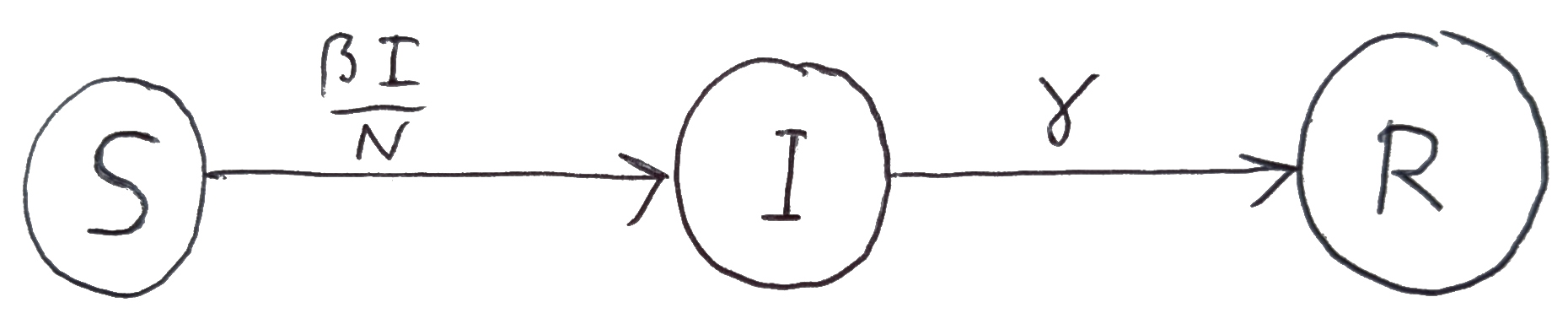
The population of size \(N\) is divided into three compartments: susceptible (\(S\)), infected and infectious (\(I\)), and recovered and immune (\(R\)). The last is sometimes called “removed”, since it can also include people who have died: \[ \frac{dS}{dt}=-\beta\frac{SI}{N},\qquad \frac{dI}{dt}=\beta\frac{SI}{N}-\gamma I,\qquad \frac{dR}{dt}=\gamma I. \tag{8.1}\]

Flow diagram of the SIR model. The arrows are labelled by the per-capita rates.

Group task: pooling the launch results

Agree on the meaning and the units of \(\beta\) and \(\gamma\). What is the mean time an individual stays infectious?
What was your rule for when an epidemic occurs? Express it as a single dimensionless combination of the parameters.
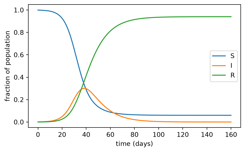
What fraction escaped infection in your simulations? What was \(S\) at the peak?

Explain: the threshold

Initially \(S(0)=S_0\approx N\), \(I(0)=I_0\ll N\) and \(R(0)=0\).

Show that \(dN/dt=0\). Which assumptions does this encode?
An epidemic starts if \(dI/dt>0\) at \(t=0\). Show that this happens iff \[R_0:=\frac{\beta S_0}{\gamma N}>1. \tag{8.2}\]
Explain why \(R_0\) is the expected number of secondary infections caused by one infected individual at the start. Compare with the reproduction number of week 7.
List three ways in which an epidemic can come about in a population where there was none.
At the start of an epidemic \(S\approx N\). Show that \(I(t)\approx I_0e^{(\beta-\gamma)t}\) and find the doubling time.

Check: feedback quiz 8.1

You will be asked to formulate compartmental models from verbal descriptions, compute \(R_0\), and compute initial growth rates and doubling times.

Consolidation: threshold and early growth

\(\beta\) is the transmission rate (effective contacts per unit time) and \(\gamma\) the recovery rate, so \(1/\gamma\) is the mean infectious period. The SIR model assumes a fixed, well-mixed population (the infection rate \(\beta SI/N\) is mass-action), no births or deaths, no latent period, constant rates and permanent immunity.

The basic reproduction number \(R_0=\beta S_0/(\gamma N)\) is the rate of new infections caused by one infective (\(\beta S_0/N\)) times the mean duration of infection (\(1/\gamma\)). An epidemic occurs iff \(R_0>1\). It is a number, not a rate, so do not call it the “basic reproductive rate” (and do not confuse it with \(R(0)\)). An epidemic can start if

the transmission rate \(\beta\) increases (a new variant, changes in behaviour);
the recovery rate \(\gamma\) decreases (longer infectious periods);
the proportion \(S_0/N\) of susceptibles increases (waning immunity, births, a stopped vaccination programme).

Early on, \(I\approx I_0e^{(\beta-\gamma)t}\) with doubling time \(t_d=\ln2/(\beta-\gamma)\). For \(\beta=0.3\) and \(\gamma=0.1\) per day, \(R_0\approx3\) and \(t_d\approx3.5\) days.

8.2 How an epidemic unfolds

The SIR equations cannot be solved in closed form, but we can find the shape of the trajectories and hence the two numbers that matter most: how many people are ill at the peak and how many are infected in total.

Explain: the trajectory in the \(S\)–\(R\) plane

Show that \(\dfrac{dS}{dR}=-\dfrac{\beta}{\gamma N}S\) and hence \[S=S_0\exp\left(-\frac{\beta}{\gamma N}R\right).\]
Why does this imply that \(S\) never reaches zero?
At the end of the epidemic \(I=0\). Show that \(S_\infty=S(\infty)\) satisfies the final-size equation \[S_\infty=S_0\exp\left(-\frac{\beta}{\gamma N}(N-S_\infty)\right). \tag{8.3}\]

Explain: the trajectory in the \(S\)–\(I\) plane

Show that \(\dfrac{dI}{dS}=-1+\dfrac{\gamma N}{\beta S}\) and integrate to get \[I=N-S+\frac{\gamma N}{\beta}\ln\frac{S}{S_0}\] (using \(S_0+I_0=N\)).
Show that the peak of the epidemic occurs when \(S=\gamma N/\beta\) and that \[I_{\max}=N-\frac{S_0}{R_0}\left(1+\ln R_0\right).\]
Interpret the condition \(S=\gamma N/\beta\) in terms of the effective reproduction number \(R_t=\beta S(t)/(\gamma N)\).

Explore: notebook part B

For several values of \(\beta\) and \(\gamma\), compare the simulated \(I_{\max}\) and \(S_\infty\) with your formulas. (Part B solves the final-size equation numerically.)
Plot the fraction ever infected, \(1-S_\infty/N\), against \(R_0\). How large is the epidemic for \(R_0=1.5\)? For \(R_0=3\)?
The peak happens when \(R_t=1\), but the epidemic continues after the peak. How many more people get infected after the peak? Explain this “overshoot”.

Group task: planning for the peak

A new influenza strain has \(R_0=1.8\) in a city of one million people. 5% of those infected need a hospital bed for an average of 5 days, and a person is infectious for an average of 3 days.

Estimate the number of people infected at the peak and the total number infected.
Estimate the maximum number of hospital beds occupied at the same time. What simplifying assumption did you make?
Use the notebook to check your estimates.

Check: feedback quiz 8.2

You will be asked to compute the peak number of infecteds, set up the final-size equation, and interpret the trajectories of the SIR model.

Consolidation: peak and final size

Along trajectories: \[ S=S_0e^{-\beta R/(\gamma N)},\qquad I=N-S+\frac{\gamma N}\beta\ln\frac S{S_0}. \] The number of infecteds peaks when \(S=\gamma N/\beta\), i.e. when the effective reproduction number \(R_t=\beta S/(\gamma N)\) drops to \(1\). The peak is \(I_{\max}=N-\frac{S_0}{R_0}(1+\ln R_0)\). The epidemic ends with \(S_\infty>0\), where \(S_\infty\) solves the transcendental final-size equation Eq. 8.3. So some people always escape infection, because the epidemic runs out of infectives before it runs out of susceptibles. For \(S_0\approx N\) and \(s=S_\infty/N\) the equation reads \(s=e^{-R_0(1-s)}\). With \(R_0=3\) about 94% of the population is infected, and the peak is about 30% of the population. After the peak, \(R_t<1\) but the remaining infecteds still cause further infections, so the final size is well beyond the herd-immunity level \(1-1/R_0\) (the overshoot).

Figure 8.1: An SIR epidemic with \(N=1000\), \(I_0=1\), \(\beta=0.3\), \(\gamma=0.1\) per day.

8.3 Vaccination and herd immunity

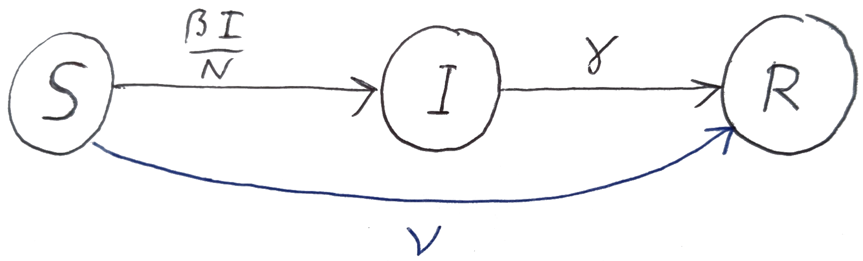
Vaccination moves individuals directly from \(S\) to \(R\).

Predict

A disease has \(R_0=4\) in an unvaccinated population. What fraction of the population must be vaccinated in advance to prevent an epidemic? What about measles, with \(R_0\approx15\)?

Explain: herd immunity

A fraction \(p\) of the population is immune before the disease arrives, so \(S_0=(1-p)N\). Using Eq. 8.2, find the critical fraction \(p_c\) above which no epidemic can occur. Express it in terms of \(\beta/\gamma\).
Why does vaccinating a fraction \(p_c\) also protect the unvaccinated?

Explore: notebook part C

Part C adds vaccination during the epidemic at per-capita rate \(\nu\): \[ \frac{dS}{dt}=-\beta\frac{SI}N-\nu S,\qquad \frac{dI}{dt}=\beta\frac{SI}N-\gamma I,\qquad \frac{dR}{dt}=\gamma I+\nu S. \]

How does the vaccination rate affect the peak and the final size?
Does vaccination change the value of \(S\) at which the peak occurs? Why?
The notebook also lets you set an initial immune fraction \(R(0)\). Check your herd-immunity threshold.

Check: feedback quiz 8.3

You will be asked to calculate herd-immunity thresholds and the effect of vaccination on \(R_0\).

Consolidation: vaccination

Pre-vaccinating a fraction \(p\) gives \(R_0=(1-p)\beta/\gamma\), so an epidemic is prevented if \[ p>p_c=1-\frac{\gamma}{\beta}. \] For \(\beta/\gamma=4\), \(p_c=75\%\). For measles, \(p_c\approx93\%\). This is herd immunity: with enough immune people, each infective infects on average fewer than one other, so the chains of transmission die out and the unvaccinated are protected too.

Vaccination during an epidemic at rate \(\nu\) does not change \(dI/dt\), so the peak still occurs at \(S=\gamma N/\beta\). But since \(S\) is removed faster, the peak comes sooner and is lower. One finds \(I_{\max}+\frac{\nu N}{\beta}\ln\frac{I_{\max}}{I_0}=I_{\max}(\nu=0)\).

8.4 Loss of immunity and endemic diseases

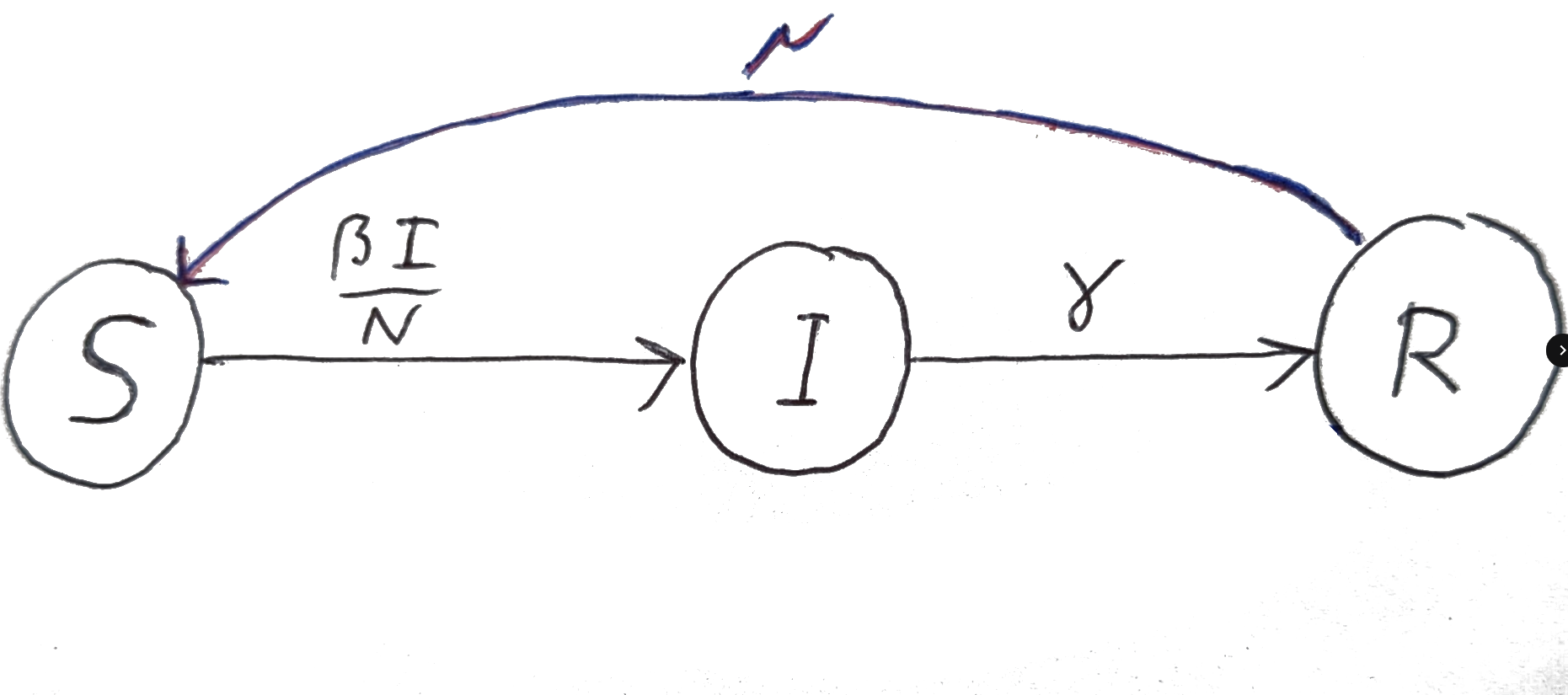
For many diseases immunity wanes over time. We add a flow from \(R\) back to \(S\) at per-capita rate \(\mu\): \[ \frac{dS}{dt}=-\beta\frac{SI}N+\mu R,\qquad \frac{dI}{dt}=\beta\frac{SI}N-\gamma I,\qquad \frac{dR}{dt}=\gamma I-\mu R. \tag{8.4}\]

Explore: notebook part D

With \(\mu>0\), what happens in the long run? Try a long final time.
How do the long-term values of \(S\), \(I\) and \(R\) depend on \(\beta\), \(\gamma\) and \(\mu\)? Which of them does not depend on \(\mu\)?
How is the long-term state approached?

Explain: the endemic state

Find the disease-free steady state and the endemic steady state \((S^*,I^*,R^*)\) with \(I^*>0\). When does the endemic state exist?
Use \(S=N-I-R\) to reduce the model to two equations for \(I\) and \(R\), and compute the Jacobian.
Classify the disease-free state.
At the endemic state use \(\beta S^*/N=\gamma\) to simplify the Jacobian to \[A=\begin{pmatrix}-\beta I^*/N&-\beta I^*/N\\ \gamma&-\mu\end{pmatrix}\] and show that the endemic state is stable whenever it exists.

Check: feedback quiz 8.4

You will be asked to find disease-free and endemic steady states of SIR variants and to determine their stability.

Consolidation: endemic equilibrium

The disease-free state is \((N,0,0)\). The endemic state has \[ S^*=\frac{\gamma}{\beta}N,\qquad I^*=N\frac{1-\gamma/\beta}{1+\gamma/\mu},\qquad R^*=\frac{\gamma}{\mu}I^*, \] and exists iff \(\beta>\gamma\), i.e. \(R_0>1\). At the disease-free state the Jacobian of the \((I,R)\) system has eigenvalues \(\beta-\gamma\) and \(-\mu\). So the disease-free state is stable if \(R_0<1\) and a saddle if \(R_0>1\). At the endemic state \(\operatorname{tr}A=-\beta I^*/N-\mu<0\) and \(\det A=\frac{\beta I^*}N(\mu+\gamma)>0\), so it is stable, typically a stable spiral: the disease settles to the endemic level through damped waves of infection. Note that \(S^*=N/R_0\) is independent of \(\mu\): at equilibrium each infective replaces itself exactly once.

8.5 Exam-style questions

Exam-style question 8.1: vaccination and loss of immunity

Consider the SIR model with vaccination at per-capita rate \(\nu\) and loss of immunity at per-capita rate \(\mu\).

Write down the ODEs for \(S\), \(I\) and \(R\). [2 marks]
Find the disease-free steady state. [2 marks]
Find the endemic steady state and the condition for its existence. [4 marks]
Viewing the model as a two-dimensional system for \(I\) and \(R\), find the Jacobian and classify both steady states. [6 marks]

Solution

\(\dot S=-\beta SI/N-\nu S+\mu R\), \(\dot I=\beta SI/N-\gamma I\), \(\dot R=\gamma I+\nu S-\mu R\).
\(I^*=0\) and \(\nu S^*=\mu R^*\) with \(S^*+R^*=N\): \(S^*=\frac{\mu}{\mu+\nu}N\), \(R^*=\frac{\nu}{\mu+\nu}N\).
\(\dot I=0\) with \(I>0\) gives \(S^*=\gamma N/\beta\). Then \(\dot S=0\) with \(R=N-S-I\) gives \(0=-\gamma I^*-\nu\frac{\gamma}{\beta}N+\mu\left(N-I^*-\frac\gamma\beta N\right)\), so \[I^*=\frac{N}{\gamma+\mu}\left(\mu-(\mu+\nu)\frac\gamma\beta\right).\] This is positive iff \(\frac{\beta}{\gamma}\frac{\mu}{\mu+\nu}>1\) (and then \(R^*>0\) too).
With \(S=N-I-R\): \(\dot I=\beta(N-I-R)I/N-\gamma I\) and \(\dot R=(\gamma-\nu)I-(\mu+\nu)R+\nu N\). So \(A=\begin{pmatrix}\beta(N-2I-R)/N-\gamma&-\beta I/N\\ \gamma-\nu&-(\mu+\nu)\end{pmatrix}\). At the disease-free state \(A\) is lower triangular with eigenvalues \(\frac{\beta\mu}{\mu+\nu}-\gamma\) and \(-(\mu+\nu)\). It is stable if \(\frac\beta\gamma\frac{\mu}{\mu+\nu}<1\) and a saddle otherwise. At the endemic state \(A=\begin{pmatrix}-\beta I^*/N&-\beta I^*/N\\ \gamma-\nu&-(\mu+\nu)\end{pmatrix}\), with \(\operatorname{tr}<0\) and \(\det=\frac{\beta I^*}{N}(\mu+\gamma)>0\): stable.

Exam-style question 8.2: initial immunity

Repeat the analysis of Section 8.2 for the case where initially a number \(R(0)=R_i>0\) of individuals are already immune, so that \(S_0+I_0+R_i=N\). Find the threshold condition, the trajectory \(I(S)\), the peak \(I_{\max}\) and the final-size equation. [8 marks]

Solution

The threshold is unchanged in form: an epidemic occurs iff \(\beta S_0/(\gamma N)>1\), but now \(S_0=N-I_0-R_i\) is smaller. From \(dS/dR=-\beta S/(\gamma N)\): \(S=S_0e^{-\beta(R-R_i)/(\gamma N)}\). From \(dI/dS=-1+\gamma N/(\beta S)\): \(I=I_0+S_0-S+\frac{\gamma N}{\beta}\ln\frac S{S_0}\). The peak is still at \(S=\gamma N/\beta\), so \(I_{\max}=I_0+S_0-\frac{\gamma N}\beta\left(1+\ln\frac{\beta S_0}{\gamma N}\right)\). At the end \(R_\infty=N-S_\infty\), so \(S_\infty=S_0\exp\left(-\frac{\beta}{\gamma N}(N-S_\infty-R_i)\right)\).

Exam-style question 8.3: recrudescence

In some diseases the pathogen stays dormant after recovery and can reactivate. Model this by a flow from \(R\) back to \(I\) at per-capita rate \(\delta\).

Write down the model and find the endemic state. [4 marks]
Is the endemic state stable for all positive parameter values? [5 marks]

Solution

\(\dot S=-\beta SI/N\), \(\dot I=\beta SI/N-\gamma I+\delta R\), \(\dot R=\gamma I-\delta R\). With \(I^*>0\), \(\dot S=0\) forces \(S^*=0\). Then \(R^*=\gamma I^*/\delta\) and \(I^*+R^*=N\) give \(I^*=\frac{\delta N}{\delta+\gamma}\).
With \(S=N-I-R\) the Jacobian of the \((I,R)\) system is \(\begin{pmatrix}\frac\beta N(N-2I-R)-\gamma&\delta-\frac{\beta I}N\\ \gamma&-\delta\end{pmatrix}\), which at the endemic state (where \(N-I^*-R^*=0\)) is \(\begin{pmatrix}-\frac{\beta I^*}N-\gamma&\delta-\frac{\beta I^*}N\\ \gamma&-\delta\end{pmatrix}\). Then \(\operatorname{tr}<0\) and \(\det=(\delta+\gamma)\beta I^*/N>0\): stable for all positive parameters.

Exam-style question 8.4: reinfection or loss of immunity?

Instead of losing immunity, suppose recovered individuals can be reinfected directly, moving from \(R\) to \(I\) at per-capita rate \(\mu\beta I/N\). Find the number of infecteds in the endemic state and compare with the model with loss of immunity. Is the effect the same? [6 marks]

Solution

\(\dot S=-\beta SI/N\), \(\dot I=\beta SI/N-\gamma I+\mu\beta RI/N\), \(\dot R=\gamma I-\mu\beta RI/N\). With \(I^*>0\): \(S^*=0\) and \(R^*=\gamma N/(\beta\mu)\), so \(I^*=N\left(1-\frac{\gamma}{\beta\mu}\right)\). This differs from \(I^*=N\frac{1-\gamma/\beta}{1+\gamma/\mu}\) for loss of immunity. In particular no susceptibles remain, and the endemic state needs \(\beta\mu>\gamma\). The two mechanisms are not equivalent.

Exam-style question 8.5: a sex-structured SIR model

For a sexually transmitted disease, males (\(S,I,R\)) and females (\(S',I',R'\)) satisfy \[ \dot S=-rSI',\quad \dot I=rSI'-aI,\quad \dot R=aI,\qquad \dot S'=-r'S'I,\quad \dot I'=r'S'I-a'I',\quad \dot R'=a'I', \] with \(R(0)=R'(0)=0\).

Show that \(N=S+I+R\) and \(N'=S'+I'+R'\) are constant. [1 mark]
Show that \(S=S_0e^{-rR'/a'}\) and find a similar equation for \(S'\). [3 marks]
Assuming \(I,I'\to0\), find two equations that determine \(S(\infty)\) and \(S'(\infty)\). [3 marks]

Solution

Adding the equations gives \(\dot N=0\) and \(\dot N'=0\).
\(\frac{dS}{dR'}=\frac{-rSI'}{a'I'}=-\frac r{a'}S\), so \(S=S_0e^{-rR'/a'}\). Similarly \(S'=S'_0e^{-r'R/a}\).
At \(t=\infty\), \(R'=N'-S'(\infty)\) and \(R=N-S(\infty)\), so \(S(\infty)=S_0e^{-\frac r{a'}(N'-S'(\infty))}\) and \(S'(\infty)=S'_0e^{-\frac{r'}{a}(N-S(\infty))}\).

Summary

SIR model: \(\dot S=-\beta SI/N\), \(\dot I=\beta SI/N-\gamma I\), \(\dot R=\gamma I\).
Threshold: an epidemic occurs iff \(R_0=\beta S_0/(\gamma N)>1\). Initial growth is \(e^{(\beta-\gamma)t}\) and the doubling time is \(\ln2/(\beta-\gamma)\).
Trajectories: \(S=S_0e^{-\beta R/(\gamma N)}\). The peak occurs at \(S=\gamma N/\beta\) and \(I_{\max}=N-\frac{S_0}{R_0}(1+\ln R_0)\). The final size follows from the transcendental equation Eq. 8.3, and some always escape.
Herd immunity: vaccinating a fraction \(p>1-\gamma/\beta\) prevents epidemics.
Loss of immunity leads to a stable endemic state with \(S^*=\gamma N/\beta\).

8.6 Launch: spreading in space

Launch investigation for week 9

Open the week 9 notebook in Colab

So far we have ignored where individuals are. Animals move, and when they move randomly the population spreads out.

In part A of the notebook, 2000 “random walkers” each step left or right at random. Predict: how does the typical distance from the starting point grow with time: linearly, like \(\sqrt t\), or some other way?
Run the simulation and check your prediction using the mean squared distance. How does it depend on the step length and the time between steps?
Compare the histogram of walker positions with the curve drawn by the notebook, which is a solution of the diffusion equation \(\partial_tu=D\,\partial_x^2u\). How is \(D\) related to the step length and the time between steps?
Bring your observations to the first session of week 9.