7 Age structure and reproduction numbers
Last week we found that an age-structured population typically settles into a stable age distribution and grows by the factor given by the dominant eigenvalue of its Leslie matrix. This week we find out when that is guaranteed, and discover a much simpler criterion for whether a population grows or dies out: the reproduction number, the expected number of offspring of an individual over its lifetime. We then move from discrete to continuous age, which leads to our first partial differential equation. The reproduction number will reappear as the famous \(R_0\) of epidemiology next week.
By the end of this week you should be able to:
- draw the Leslie graph of a Leslie matrix and decide whether it is irreducible and primitive;
- state the Perron–Frobenius theorem for Leslie matrices and use it to predict long-term behaviour;
- derive the Euler–Lotka equation and use the reproductive number \(R\) to decide between growth and extinction;
- derive the McKendrick–von Foerster equation and solve it by separation of variables;
- apply the continuous Euler–Lotka equation to given birth and death rates.
Open the week 7 notebook in Colab
7.1 When does the age distribution settle down?
Pool your results from the launch investigation.
- What happened to the semelparous population (reproduction only at age 3)? Describe the long-term behaviour. What are the eigenvalues of its Leslie matrix and their absolute values?
- For which sets of reproductive ages did the age distribution settle down? Agree on a conjecture.
To state the answer we represent a Leslie matrix by a directed graph. The Leslie graph has one node for each age class, and an arrow from node \(i\) to node \(j\) whenever \(L_{ji}\neq0\). So there is an arrow \(a\to a+1\) for each survival probability and an arrow \(a\to0\) for each non-zero fecundity \(F_a\).
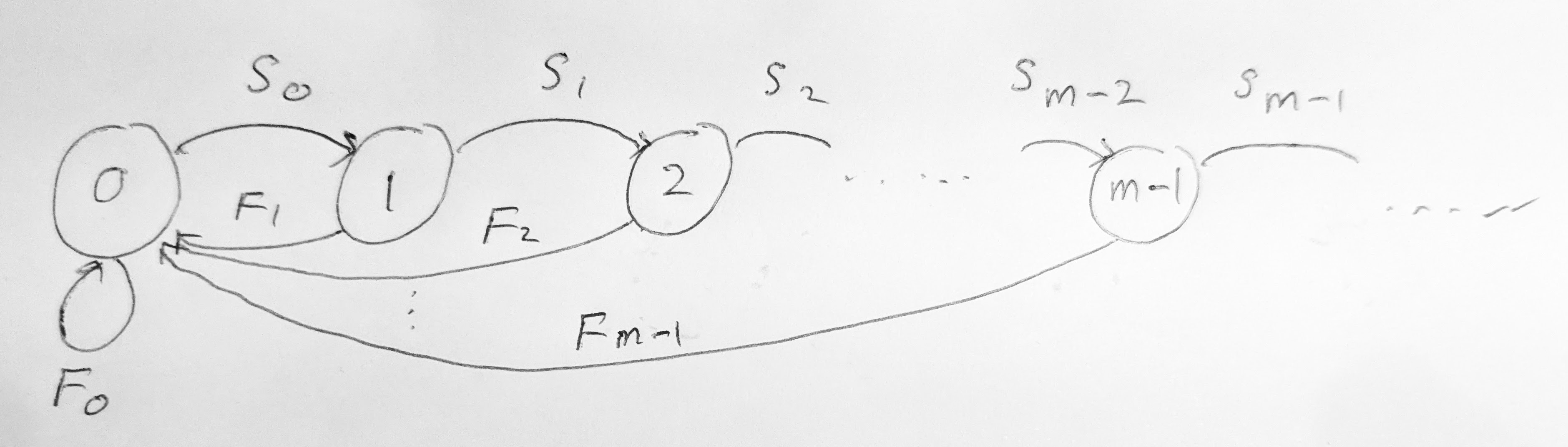
A Leslie matrix is irreducible if its Leslie graph is strongly connected: there is a directed path from every node to every other node.
It is primitive if the greatest common divisor of the lengths of all cycles (closed directed paths) in its Leslie graph is \(1\).
If a Leslie matrix is irreducible and primitive, it has a unique dominant eigenvalue \(\lambda_1\), which is real and positive, and whose eigenvector is strictly positive. Then \(\mathbf N_t/\lambda_1^t\to c_1\mathbf v_1\) for every non-zero initial condition \(\mathbf N_0\geq0\).
- What are the lengths of the cycles in a Leslie graph? Relate them to the ages at which individuals reproduce.
- Explain why the Leslie matrix of Eq. 6.2, with \(F_{m-1}>0\), is always irreducible.
- Use the theorem to explain your launch results.
- For the semelparous population, show that the eigenvalues satisfy \(\lambda^3=F_2S_0S_1\). Why do they all have the same absolute value, and why does this produce oscillations with period 3?
You will be asked to decide from a life table or a Leslie matrix whether it is irreducible and primitive, and whether the population approaches a stable age distribution.
Every cycle in a Leslie graph goes \(0\to1\to\cdots\to a\to0\) and uses a non-zero fecundity \(F_a=b_{a+1}S_a\). Its length is \(a+1\), an age at which individuals reproduce. So a Leslie matrix is primitive iff the reproductive ages have no common divisor larger than 1. Any two consecutive reproductive ages suffice, as does reproduction at age 1 or a plus group (a self-loop of length 1). If the last age class reproduces, every node can reach \(0\) and \(0\) can reach every node, so the matrix is irreducible.
For a semelparous population reproducing only at age 3 the cycle length is 3, and the eigenvalues solve \(\lambda^3=F_2S_0S_1\). They are the three cube roots, all with the same modulus, so none is dominant. The population cycles with period 3: \((10,0,0)\to(0,10,0)\to(0,0,5)\to(10,0,0)\) in the launch example. Periodical cicadas, which emerge every 13 or 17 years, are a striking real example of such cohort cycles.
7.2 The reproduction number
The eigenvalue problem gives \(\lambda_1\), but computing eigenvalues of large matrices by hand is hard. Luckily, deciding between growth and extinction is much easier.
Let \(l_a=S_0S_1\cdots S_{a-1}\) (with \(l_0=1\)) be the probability of surviving from birth to age \(a\). We look for a solution with a stable age distribution, \(N_{a,t+1}=\lambda N_{a,t}\) for all \(a\).
- Show that \(N_{a,t}=\dfrac{l_a}{\lambda^a}N_{0,t}\).
- Newborns in year \(t\) are produced by individuals reaching age \(a\), so \(N_{0,t}=\sum_{a\geq1}b_aN_{a,t}\). Deduce the Euler–Lotka equation \[1=\sum_{a\geq1}b_al_a\lambda^{-a}=:\psi(\lambda).\]
- Show that \(\psi\) is decreasing for \(\lambda>0\). Why does this mean that there is exactly one positive solution?
- Interpret \(R=\psi(1)=\sum_ab_al_a\). Show that \(\lambda>1\) iff \(R>1\).
Part B contains the life tables of the Eastern screech owl in suburban and rural Texas. The table gives \(l_a\) (survival from birth to age \(a\)) and \(b_a\).
- Before running the notebook, compute \(R\) for both habitats by hand. Which population grows?
- Use the notebook to find \(\lambda\) from the Euler–Lotka equation and from the Leslie matrix. Do they agree?
- \(R\) and \(\lambda\) are both “growth factors”. What is the difference between them? Why is \(R\) further from 1 than \(\lambda\)?
You will be asked to compute survival functions \(l_a\) and reproduction numbers \(R\) from life tables, set up the Euler–Lotka equation and solve it in simple cases.
A population with a stable age distribution has \(N_{a,t}=\lambda^{t-a}l_aN_{0,0}\), and \(\lambda\) solves the Euler–Lotka equation \[ \psi(\lambda)=\sum_{a\geq1}b_al_a\lambda^{-a}=1. \tag{7.1}\] Since \(\psi\) is strictly decreasing from \(+\infty\) to \(0\), there is a unique positive solution, and it equals the dominant eigenvalue of the Leslie matrix. The reproduction number \[ R=\psi(1)=\sum_{a\geq1}b_al_a \] is the expected number of offspring produced by a newborn over its whole lifetime. Since \(\psi\) is decreasing,
- \(R>1\iff\lambda>1\): the population grows;
- \(R<1\iff\lambda<1\): the population goes extinct.
\(R\) is a growth factor per generation and \(\lambda\) a growth factor per year. Roughly \(R\approx\lambda^{T_g}\), where \(T_g\) is the generation time. For the screech owls, \(R\approx1.04\) in suburbs (slow growth) and \(R\approx0.52\) in rural areas (decline).
7.3 Continuous age: the McKendrick–von Foerster equation
For species that reproduce throughout the year we describe the population by a density \(n(t,a)\): the number of individuals with ages between \(a_1\) and \(a_2\) at time \(t\) is \(\int_{a_1}^{a_2}n(t,a)\,da\). Individuals die at the age-dependent rate \(\mu(a)\) and give birth at the rate \(b(a)\).
- In a short time \(\delta t\), the individuals of age \(a\) become individuals of age \(a+\delta t\), and a fraction \(\mu(a)\delta t\) of them die. Explain why \[n(t+\delta t,a+\delta t)=n(t,a)-\mu(a)n(t,a)\delta t.\]
- Taylor expand the left-hand side and take \(\delta t\to0\) to obtain the McKendrick–von Foerster equation \[\frac{\partial n}{\partial t}+\frac{\partial n}{\partial a}=-\mu(a)n. \tag{7.2}\]
- Newborns have age \(0\). Explain the boundary condition \[n(t,0)=\int_0^\infty b(a)n(t,a)\,da. \tag{7.3}\] Why are the units of \(n(t,0)\) and \(b(a)\) different from those of \(N_{0,t}\) and \(b_a\) in the discrete model?
Part C solves the McKendrick–von Foerster equation numerically, starting from an age distribution of your choice. It plots the age distribution (normalised to total 1) at several times and the total population.
- Does the age distribution settle down? Does the final shape depend on the initial distribution?
- With constant rates \(\mu\) and \(b\), how does the long-term growth rate depend on \(b\) and \(\mu\)? What does the final age distribution look like?
- Try an age-dependent birth rate, e.g. reproduction only between ages 1 and 3.
- Substitute \(n(t,a)=f(t)r(a)\) into Eq. 7.2 and separate variables with a separation constant \(\gamma\). Solve both ODEs to obtain \[n(t,a)=n(0,0)\,l(a)\,e^{\gamma(t-a)},\qquad l(a)=\exp\left(-\int_0^a\mu(a')\,da'\right).\] Interpret \(l(a)\).
- Substitute into Eq. 7.3 to obtain the continuous Euler–Lotka equation \[1=\int_0^\infty b(a)l(a)e^{-\gamma a}\,da=:\phi(\gamma).\]
- Show that \(\phi\) is decreasing, and deduce that the population grows iff \(R=\phi(0)=\int_0^\infty b(a)l(a)\,da>1\).
- For constant \(b\) and \(\mu\), find \(l(a)\), \(\phi(\gamma)\), \(\gamma\) and \(R\). Compare with the exponential model of week 1 and with your observations.
You will be asked to compute \(l(a)\) and \(R\) for given \(\mu(a)\) and \(b(a)\), to state conditions for persistence, and to solve the Euler–Lotka equation in simple cases.
The age density satisfies \[ \partial_tn+\partial_an=-\mu(a)n,\qquad n(t,0)=\int_0^\infty b(a)n(t,a)\,da. \] Separable solutions have a stable age distribution, \(n(t,a)=n(0,0)\,l(a)e^{\gamma(t-a)}\), where the survival function \(l(a)=e^{-\int_0^a\mu}\) is the probability of reaching age \(a\), and \(\gamma\) is the unique real root of the continuous Euler–Lotka equation \[ \phi(\gamma)=\int_0^\infty b(a)l(a)e^{-\gamma a}\,da=1. \tag{7.4}\] \(\phi\) is strictly decreasing, so with \(R=\phi(0)=\int_0^\infty b(a)l(a)\,da\), the population grows (\(\gamma>0\)) iff \(R>1\) and declines iff \(R<1\). As in discrete time, general solutions converge to the stable age distribution.
For constant rates, \(l(a)=e^{-\mu a}\), \(\phi(\gamma)=b/(\mu+\gamma)\), \(\gamma=b-\mu\) and \(R=b/\mu\). This is the exponential model, and the stable age distribution is exponential, \(\propto e^{-ba}\).
7.4 Exam-style questions
A population reproduces once, when individuals turn 3, and not before or after. Draw its Leslie graph. Is the Leslie matrix irreducible? Is it primitive? What does this mean for the long-term behaviour? [4 marks]
Individuals produce one offspring when they turn 1 and another when they turn 2, and then die. All individuals survive to age 1, but only half survive to age 2. Write down the Leslie matrix, compute the population at \(t=1,2,3,4\) starting with 20 newborns, draw the Leslie graph, decide whether the matrix is irreducible and primitive, and find the long-term growth factor. [8 marks]
Nodes \(0,1,2\) with arrows \(0\to1\to2\to0\) (the last from \(F_2=b_3S_2\)). The graph is strongly connected, so irreducible. The only cycle has length 3, so it is not primitive. There is no unique dominant eigenvalue, and the population oscillates with period 3 rather than settling to a stable age distribution.
\(b_1=b_2=1\), \(S_0=1\), \(S_1=1/2\), so \(F_0=b_1S_0=1\) and \(F_1=b_2S_1=1/2\): \(L=\begin{pmatrix}1&1/2\\1&0\end{pmatrix}\). \(\mathbf N_0=(20,0)\), \(\mathbf N_1=(20,20)\), \(\mathbf N_2=(30,20)\), \(\mathbf N_3=(40,30)\), \(\mathbf N_4=(55,40)\). The graph has arrows \(0\to0\), \(0\to1\), \(1\to0\), with cycles of lengths 1 and 2. It is irreducible and primitive. \(\lambda^2-\lambda-\frac12=0\) gives \(\lambda_1=\frac{1+\sqrt3}{2}\approx1.366\).
For the spotted owl, \(b_a=0\) for \(a<2\) and \(b_a=b\) for \(a\geq2\). The survival probabilities are \(S_0=1\), \(S_1=l\) and \(S_a=p\) for \(a\geq2\), with \(0<p<1\).
Find the probability \(l_a\) of surviving from birth to age \(a\). [2 marks]
Find the expected lifetime number of offspring and the condition on \(b\) for the population to persist. [3 marks]
Find the long-term growth factor and the stable age distribution. [5 marks]
\(l_1=1\) and \(l_a=lp^{a-2}\) for \(a\geq2\).
\(R=\sum_{a\geq2}blp^{a-2}=\dfrac{bl}{1-p}\). The population persists iff \(R>1\), i.e. \(b>(1-p)/l\).
\(\psi(\lambda)=bl\sum_{a\geq2}p^{a-2}\lambda^{-a}=\dfrac{bl}{\lambda(\lambda-p)}\) for \(\lambda>p\). Then \(\psi(\lambda)=1\) gives \(\lambda^2-p\lambda-bl=0\), so \(\lambda=\frac{p+\sqrt{p^2+4bl}}{2}\). The stable age distribution is \(N_{a,t}=\lambda^{t-a}l_aN_{0,0}\).
In the continuous-time age-structured model the mortality rate is \(\mu(a)=a\) and the birth rate is \(b(a)=ra\) for \(1\leq a<3\) and \(0\) otherwise, where \(r>0\).
Find the probability of surviving to age \(a\). [2 marks]
Find the expected lifetime number of offspring. [3 marks]
Give the condition on \(r\) for the population to persist. [1 mark]
You may use results derived in the learning guide without proof.
\(l(a)=e^{-\int_0^aa'\,da'}=e^{-a^2/2}\).
\(R=\int_1^3rae^{-a^2/2}\,da=r\left[-e^{-a^2/2}\right]_1^3=r\left(e^{-1/2}-e^{-9/2}\right)\).
Persistence iff \(R>1\), i.e. \(r>1/(e^{-1/2}-e^{-9/2})\approx1.68\).
In the continuous-time model take \(b(a)=b\) and \(\mu(a)=\mu\) constant. Solve the McKendrick–von Foerster equation by separation of variables, use the boundary condition to find the separation constant, and give the condition for extinction. Compare with the exponential model. [8 marks]
With \(n=f(t)r(a)\): \(f'/f=-r'/r-\mu=\gamma\), so \(f=f(0)e^{\gamma t}\) and \(r=r(0)e^{-(\gamma+\mu)a}\), giving \(n=n(0,0)e^{\gamma t-(\gamma+\mu)a}\). The boundary condition gives \(1=\int_0^\infty be^{-(\gamma+\mu)a}\,da=\frac{b}{\gamma+\mu}\), so \(\gamma=b-\mu\). The population goes extinct iff \(b<\mu\), exactly as in the exponential model \(dN/dt=(b-\mu)N\) (integrate the PDE over \(a\) to see this directly).
In addition to age-dependent mortality there is a seasonal mortality \(m(t)\): \[ \partial_tn+\partial_an=-(\mu(a)+m(t))n,\qquad n(t,0)=\int_0^\infty b(a)n(t,a)\,da. \]
With \(n(t,a)=p(t)r(a)\) and separation constant \(\gamma\), find \(p\), \(r\) and \(n\). [4 marks]
Derive an equation \(\phi(\gamma)=1\) and show that \(\phi\) is monotonic. [3 marks]
Let \(m\) have period 1 and average \(F=\int_0^1m(t)\,dt\). By looking at the population at the end of each season, show that it goes extinct if \(\gamma<F\). [3 marks]
Hence give the condition for extinction in terms of \(b\), \(\mu\) and \(F\). [3 marks]
\(p'/p+m(t)=-r'/r-\mu(a)=\gamma\), so \(p(t)=p(0)e^{\int_0^t(\gamma-m)}\), \(r(a)=r(0)e^{-\int_0^a(\gamma+\mu)}\) and \(n=n(0,0)e^{\int_0^t(\gamma-m)}e^{-\int_0^a(\gamma+\mu)}\).
\(1=\int_0^\infty b(a)e^{-\gamma a-\int_0^a\mu}\,da=\phi(\gamma)\). The integrand decreases with \(\gamma\), so \(\phi\) is decreasing.
At integer times \(\int_0^t(\gamma-m)=t(\gamma-F)\), so \(n(t,a)=n(0,0)e^{t(\gamma-F)}r(a)/r(0)\to0\) if \(\gamma<F\).
Since \(\phi\) is decreasing and \(\phi(\gamma)=1\): \(\gamma<F\iff1>\phi(F)\). So the population goes extinct iff \(\int_0^\infty b(a)e^{-Fa-\int_0^a\mu}\,da<1\).
Summary
- Leslie graph: arrows \(a\to a+1\) (survival) and \(a\to0\) (fecundity). The matrix is irreducible if the graph is strongly connected and primitive if the gcd of the cycle lengths (the reproductive ages) is 1.
- Perron–Frobenius: irreducible and primitive implies a unique positive dominant eigenvalue and convergence to the stable age distribution.
- Euler–Lotka: \(\sum_ab_al_a\lambda^{-a}=1\) (discrete) and \(\int b(a)l(a)e^{-\gamma a}\,da=1\) (continuous).
- Reproduction number \(R=\sum b_al_a\) or \(\int b\,l\,da\): the population grows iff \(R>1\).
- McKendrick–von Foerster: \(\partial_tn+\partial_an=-\mu(a)n\) with births as a boundary condition at \(a=0\), solved by separation of variables.
7.5 Launch: an epidemic
Open the week 8 notebook in Colab
In 1927 Kermack and McKendrick (the same McKendrick as in this week’s equation) proposed a model for an epidemic in which the population is divided into susceptible (\(S\)), infected (\(I\)) and recovered (\(R\)) individuals: \[ \frac{dS}{dt}=-\beta\frac{SI}N,\qquad \frac{dI}{dt}=\beta\frac{SI}N-\gamma I,\qquad \frac{dR}{dt}=\gamma I. \]
- Before running anything: explain each term. What are the units of \(\beta\) and \(\gamma\)? Estimate the average time an individual stays infected.
- In part A of the notebook, start with one infected person in a population of
- For which combinations of \(\beta\) and \(\gamma\) is there an epidemic? Find a rule.
- Does everyone get infected? How does the number who escape infection depend on \(\beta\) and \(\gamma\)?
- At the peak of the epidemic, how many susceptibles are left? Compare this number for several parameter values and look for a pattern.