2 Harvesting and bifurcations
We harvest natural populations: we catch fish, hunt deer and cut down forests. We would like to do this sustainably, meaning in a way that can continue indefinitely, while taking as large a yield as possible. This week we use the tools of week 1 to compare two management strategies used in real fisheries. Along the way we discover what happens when a steady state appears, disappears or changes its stability as a parameter is varied: a bifurcation.
TipLearning outcomes for this week
By the end of this week you should be able to:
- add harvesting terms to a population model and interpret them;
- calculate the maximum sustainable yield for harvesting with fixed effort;
- explain why harvesting with a fixed quota can lead to sudden collapse;
- draw and interpret bifurcation diagrams, and recognise saddle-node and transcritical bifurcations;
- explain why a collapsed population may fail to recover when harvesting is reduced.
Open the week 2 notebook in Colab
2.1 Fixed effort and maximum sustainable yield
In the launch investigation (Section 1.6) you explored the model \[ \frac{dN}{dt}=rN\left(1-\frac{N}{K}\right)-EN, \tag{2.1}\] in which fish are caught at a rate \(EN\) proportional to their abundance. The constant \(E\) is set by the fishing effort (number of boats, days at sea). The rate \(Y=EN\) at which fish are caught is the yield.
WarningGroup task: pooling the launch results
Compare your tables of \(N^*\) and \(Y^*=EN^*\) from the launch investigation.
- Agree on a formula for \(N^*\) as a function of \(E\), \(r\) and \(K\).
- Agree on the effort \(E_{\text{MSY}}\) that maximises the long-term yield and on the maximal yield itself. How do they depend on \(r\) and \(K\)?
- What happens when \(E\geq r\)?
NoteExplain
- Show that Eq. 2.1 can be written as a logistic equation with growth rate \(r-E\) and carrying capacity \(K(1-E/r)\). Read off the steady states.
- For \(E<r\) determine the stability of both steady states by linearisation.
- The sustainable yield is the yield at the stable steady state, \(Y^*(E)=EN^*(E)\). Find the effort \(E_{\text{MSY}}\) that maximises it and show that the maximum sustainable yield is \(\text{MSY}=rK/4\).
- What is the population size when fishing at MSY? Relate this to the result from week 1 that the logistic growth rate is maximal at \(K/2\).
- Draw the parabola \(rN(1-N/K)\) and the straight line \(EN\) in one diagram. Explain the steady state and the MSY using this diagram.
TipExplore: notebook part A (continued)
Move the population away from its steady state (the notebook starts it at \(K\)) and watch how quickly it returns. How does this return time change as \(E\) approaches \(r\)? Explain this using the value of \(f'(N^*)\).
NoteCheck: feedback quiz 2.1
You will be asked to find the steady states and sustainable yield for a model with fixed-effort harvesting and to compute the MSY and the corresponding effort.
NoteConsolidation: fixed-effort harvesting
With fixed effort, \[ \frac{dN}{dt}=(r-E)N\left(1-\frac{N}{K(1-E/r)}\right). \] For \(E<r\) the steady states are \(0\) (unstable) and \(N^*=K(1-E/r)\) (stable, with \(f'(N^*)=-(r-E)\)). For \(E>r\) only \(0\) remains, and it is stable: the population is fished to extinction. The sustainable yield is \[ Y^*(E)=EK\left(1-\frac{E}{r}\right), \] which is maximised at \(E_{\text{MSY}}=r/2\), giving \[ \text{MSY}=\frac{rK}{4}, \qquad N^*_{\text{MSY}}=\frac{K}{2}. \] Geometrically, the steady state is where the line \(EN\) meets the growth parabola, and the yield is the height of the intersection point. That height is largest at the top of the parabola.
The recovery rate after a disturbance is \(|f'(N^*)|=r-E\). As the effort approaches \(r\), the population recovers more and more slowly. This “critical slowing down” is a warning sign of an approaching bifurcation.
2.2 Fixed quota
Mediterranean fisheries are managed mainly by controlling effort. In the North Sea and the North Atlantic, managers instead set a total allowable catch (TAC): a fixed quota \(Q\) of fish that may be landed per year, whatever the state of the stock. With logistic growth this gives \[ \frac{dN}{dt}=rN\left(1-\frac{N}{K}\right)-Q. \tag{2.2}\]
NotePredict
The quota is set at the MSY value \(Q=rK/4\) that you found above. Is this a good idea? What do you think happens if the stock is accidentally reduced (say by a bad year) below \(K/2\)?
TipExplore: notebook part B
Part B shows the growth curve \(rN(1-N/K)\), the horizontal line at height \(Q\), and solutions for several initial conditions.
- Increase \(Q\) from \(0\). What happens to the steady states?
- For \(0<Q<rK/4\), find the population size below which the population collapses. How does it depend on \(Q\)?
- What happens for \(Q>rK/4\)? How long does the collapse take, starting at \(K\)?
- Test your prediction about fishing at \(Q=rK/4\).
NoteExplain
- Find the steady states \(N^*_\pm\) of Eq. 2.2. For which \(Q\) do they exist?
- Determine their stability by linearisation (or from the graph).
- Explain why fixed-quota harvesting creates critical depensation, a threshold below which the population collapses, even though the unharvested population has no Allee effect.
WarningGroup task: advising a fisheries minister
Your group advises a fisheries minister who must choose between effort control and quota control. The fishing industry wants the largest catch possible. Prepare a three-sentence recommendation. It should mention what happens to each policy if \(r\) (which fluctuates from year to year) turns out to be 20% smaller than estimated. Be ready to present it to the class.
NoteCheck: feedback quiz 2.2
You will be asked to find the steady states for quota harvesting, the critical quota at which they disappear and the collapse threshold for a given quota.
NoteConsolidation: fixed-quota harvesting
The steady states of Eq. 2.2 are \[ N^*_\pm = \frac K2\left(1\pm\sqrt{1-\frac{4Q}{rK}}\right), \] which exist only for \(Q\leq rK/4\). The larger one, \(N^*_+\), is stable and the smaller one, \(N^*_-\), is unstable. \(N^*_-\) is a collapse threshold: any stock below it is driven to extinction in finite time. As \(Q\) increases, the two steady states approach each other and merge at \(Q=rK/4\). For larger quotas no steady state is left and the stock always collapses.
Fishing at the MSY with a fixed quota is therefore extremely risky: the steady state \(K/2\) is semi-stable and any downward perturbation leads to collapse. Even a quota somewhat below MSY leaves only a small safety margin \(N^*_+-N^*_-\). With effort control, in contrast, an overestimate of \(r\) merely reduces the stock. This is why quota-managed stocks need frequent reassessment, and why the TAC is set to zero for some depleted stocks.
2.3 Bifurcation diagrams
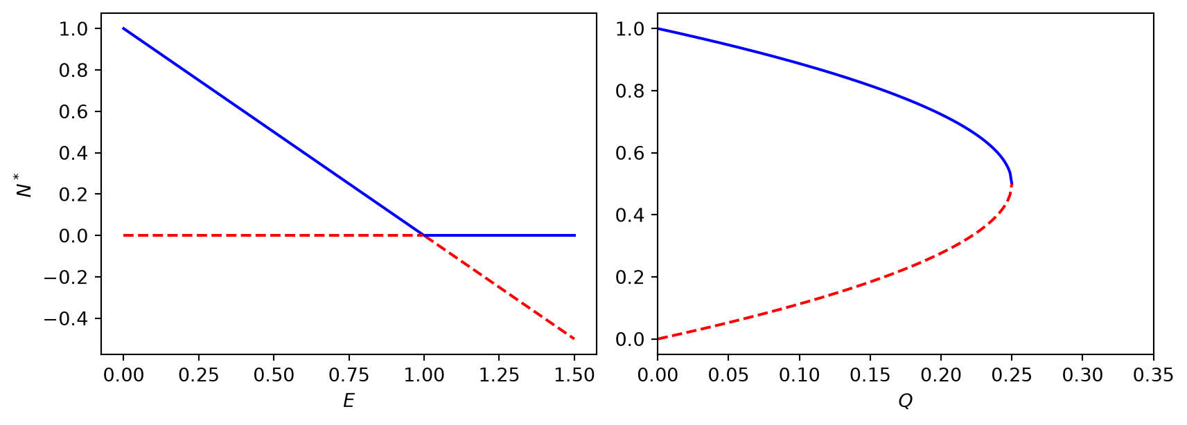
In both harvesting models the number and stability of the steady states change as a parameter is varied. A qualitative change of this kind is called a bifurcation, and the parameter value where it happens is a bifurcation point. A bifurcation diagram plots the steady states against the parameter, with stable branches drawn solid and unstable branches dashed.
NotePredict
Sketch by hand what you think the bifurcation diagrams look like for the effort model (parameter \(E\)) and for the quota model (parameter \(Q\)).
TipExplore: notebook part C
Part C draws bifurcation diagrams for any model \(dN/dt=f(N,p)\).
- Compare the diagrams for the effort model and the quota model with your sketches.
- Describe in words what happens at the bifurcation point in each case. How are the two cases different?
- Try the normal forms \(f(N,p)=p-N^2\), \(f(N,p)=pN-N^2\) and \(f(N,p)=pN-N^3\) (you need negative \(N\) for these, so change
Nmin). Which of them looks like which harvesting model?
NoteCheck: feedback quiz 2.3
You will be asked to find bifurcation points of given one-dimensional models, to identify the type of bifurcation and to match bifurcation diagrams to models.
NoteConsolidation: bifurcations of one-dimensional ODEs
At a bifurcation point of \(dN/dt=f(N,p)\) there is a steady state with \(f(N^*,p)=0\) and \(f'(N^*)=0\), because the stability can only change when \(f'(N^*)\) passes through zero. The three generic types are:
- Saddle-node bifurcation (normal form \(p-N^2\)): two steady states, one stable and one unstable, approach each other, merge and disappear. Example: the quota model at \(Q=rK/4\).
- Transcritical bifurcation (normal form \(pN-N^2\)): two steady states pass through each other and exchange stability. Example: the effort model at \(E=r\), where the branch \(K(1-E/r)\) crosses the extinction branch \(N=0\).
- Pitchfork bifurcation (normal form \(pN-N^3\)): one steady state splits into three. This needs a symmetry and is rare in population models.
You met these bifurcations in the Classical Dynamics module. We will meet them again in discrete time next week.
2.4 Tipping points: harvesting with an Allee effect
Many fish stocks that collapsed under heavy fishing have not recovered, even after fishing stopped. The best-known example is the Newfoundland cod, which collapsed in the early 1990s. One possible explanation combines harvesting with an Allee effect.
TipExplore: notebook part D
Part D simulates a population with a strong Allee effect, \[ \frac{dN}{dt}=rN\left(1-\frac{N}{K}\right)\left(\frac{N}{K_0}-1\right)-E(t)N, \] where the effort \(E(t)\) is increased slowly over 50 years and then decreased slowly back to zero.
- What happens to the population as the effort increases? Is the decline gradual or sudden?
- What happens when the effort is reduced again? Try different maximal efforts.
- Now look at the bifurcation diagram of this model in part D. Use it to explain what you saw.
WarningGroup task
- Show that the non-zero steady states satisfy \(N^2-(K+K_0)N+KK_0(1+E/r)=0\).
- Find the critical effort \(E_c\) at which the two non-zero steady states disappear. What type of bifurcation is this?
- Show that \(N=0\) is stable for every \(E\geq0\). Why does this explain the failure to recover?
- Discuss: what would a manager need to do to bring a collapsed population back?
NoteCheck: feedback quiz 2.4
You will be asked to find the critical harvesting effort at which a population with an Allee effect collapses, and to explain why it does not recover.
NoteConsolidation: tipping points and irreversibility
For the harvested Allee model the non-zero steady states are \[ N^*_\pm=\tfrac12\left(K+K_0\pm\sqrt{(K+K_0)^2-4KK_0(1+E/r)}\right), \] which exist for \(E\leq E_c=r(K-K_0)^2/(4KK_0)\). At \(E_c\) they merge in a saddle-node bifurcation, and for \(E>E_c\) the population crashes to zero. The extinction state has \(f'(0)=-r-E<0\) and is therefore stable for all efforts. Reducing the effort below \(E_c\) again brings back the steady state \(N^*_+\), but the collapsed population sits in the basin of attraction of \(0\) and does not return to \(N^*_+\). A sudden, hard-to-reverse transition at a saddle-node bifurcation is often called a tipping point. The same mathematics is used for tipping points in climate science.
2.5 Exam-style questions
ImportantExam-style question 2.1: harvesting the Gompertz model
A population is described by the Gompertz model \[ \frac{dN}{dt}=\alpha N\ln\frac KN \] with positive constants \(\alpha\) and \(K\). It is harvested with effort \(E\), so that the yield is \(Y=EN\).
Write down the ODE including the harvesting term. [1 mark]
Find the steady states and determine their stability. [4 marks]
Find the maximum sustainable yield and the effort that achieves it. [4 marks]
NoteSolution
\(\dfrac{dN}{dt}=\alpha N\ln\dfrac KN-EN=f(N)\).
For \(N>0\): \(\alpha\ln(K/N)=E\), so \(N^*=Ke^{-E/\alpha}\). Also \(N\to0\) is a steady state (in the limit, since \(N\ln(K/N)\to0\)). We have \(f'(N)=\alpha\ln(K/N)-\alpha-E\), so \(f'(N^*)=-\alpha<0\) and \(N^*\) is stable. As \(N\to0^+\), \(f'(N)\to+\infty\), so \(0\) is unstable. (Alternatively, \(f>0\) for \(0<N<N^*\) and \(f<0\) for \(N>N^*\).)
\(Y^*(E)=EKe^{-E/\alpha}\) and \(\dfrac{dY^*}{dE}=Ke^{-E/\alpha}(1-E/\alpha)=0\) gives \(E=\alpha\). So \(\text{MSY}=\alpha K/e\), achieved at \(E=\alpha\) with \(N^*=K/e\).
ImportantExam-style question 2.2: quota for the Gompertz model
Fishing is to be introduced in a lake whose fish population follows the Gompertz model of question 2.1. You must set a fixed quota \(Q\) (fish removed per unit time). The fishers demand the maximum sustainable quota. What is it, according to the model? Would it be wise to set the quota at this level? Explain using a sketch. [6 marks]
NoteSolution
With a quota, \(dN/dt=\alpha N\ln(K/N)-Q\). Steady states exist where the growth curve \(g(N)=\alpha N\ln(K/N)\) meets the horizontal line \(Q\). Since \(g'(N)=\alpha(\ln(K/N)-1)\), the maximum of \(g\) is at \(N=K/e\) with value \(\alpha K/e\). So the maximal sustainable quota is \(Q=\alpha K/e\), the same value as the MSY for effort control. At this quota the only steady state \(N^*=K/e\) is semi-stable, a saddle-node point. Any perturbation that reduces \(N\) below \(K/e\) leads to collapse. It would be unwise: the quota should be set well below \(\alpha K/e\), so that the stable steady state is well separated from the unstable threshold. The quota should also be reviewed regularly.
ImportantExam-style question 2.3: bifurcations
Consider \[ \frac{dN}{dt}=N\left(N-a\right)\left(1-N\right), \qquad N\geq0, \] where \(a\) is a real parameter. Find the steady states and their stability as a function of \(a\). Sketch the bifurcation diagram for \(-1<a<2\) and identify the bifurcations. Interpret the cases \(a<0\) and \(0<a<1\) ecologically. [8 marks]
NoteSolution
Steady states: \(0\), \(a\) (relevant if \(a\geq0\)) and \(1\). With \(f(N)=N(N-a)(1-N)\) we get \(f'(0)=-a\), \(f'(1)=-(1-a)=a-1\) and \(f'(a)=a(1-a)\). So:
- \(0\) is stable for \(a>0\) and unstable for \(a<0\);
- \(1\) is stable for \(a<1\) and unstable for \(a>1\);
- \(a\) is unstable for \(0<a<1\) and stable for \(a>1\).
There are transcritical bifurcations at \(a=0\) (the branches \(N=a\) and \(N=0\) exchange stability) and at \(a=1\) (the branches \(N=a\) and \(N=1\) exchange stability). For \(a<0\) the model is logistic-like: small populations grow to \(1\). For \(0<a<1\) there is a strong Allee effect with threshold \(a\).
ImportantExam-style question 2.4: the hornet’s dilemma
A hornet queen produces workers at rate \(rn(t)\), where \(n(t)\) is the number of workers, from time \(0\) until a switching time \(t_c\). After \(t_c\) she produces only reproductives, at rate \(Rn(t)\), until winter begins at time \(T\). There are no deaths before winter, and \(n(0)=1\). Find the number of reproductives \(N(T)\) as a function of \(t_c\), and the switching time that maximises it. [6 marks]
NoteSolution
For \(t<t_c\), \(n(t)=e^{rt}\). For \(t>t_c\) no more workers are produced and none die, so \(n=e^{rt_c}\). Then \(dN/dt=Re^{rt_c}\) gives \(N(T)=Re^{rt_c}(T-t_c)\). Differentiating with respect to \(t_c\): \(Re^{rt_c}\left(r(T-t_c)-1\right)=0\), so \(t_c=T-1/r\) (if \(T>1/r\), otherwise \(t_c=0\)). This is a maximum because the derivative changes from positive to negative.
Summary
- Fixed effort \(EN\): the steady state is \(K(1-E/r)\), and the maximum sustainable yield \(rK/4\) is achieved at \(E=r/2\), with the stock at \(K/2\). Extinction occurs via a transcritical bifurcation at \(E=r\).
- Fixed quota \(Q\): this creates critical depensation. The stable and unstable steady states merge in a saddle-node bifurcation at \(Q=rK/4\), after which the stock collapses.
- Bifurcations in 1D occur where \(f(N^*)=0\) and \(f'(N^*)=0\). The types are saddle-node, transcritical and pitchfork.
- With an Allee effect, a saddle-node bifurcation becomes a tipping point: a collapsed population does not recover when the pressure is removed.
2.6 Launch: populations with annual breeding
NoteLaunch investigation for week 3
Open the week 3 notebook in Colab
Many populations breed once a year: salmon spawn in the autumn, many birds breed in spring. It is then natural to follow the population from one year to the next, \(N_{t+1}=f(N_t)\) with \(t=0,1,2,\ldots\). A discrete-time version of the logistic model is \[ N_{t+1}=N_t+R_0N_t\left(1-\frac{N_t}{K}\right). \]
- Predict: will the population approach \(K\) in the same way as in the continuous-time logistic model?
- In part A of the notebook, look at the time series for \(R_0=0.5\), \(1.5\), \(1.9\), \(2.1\), \(2.5\) and \(2.7\). Describe each in words. Sketch any surprising ones.
- Find (roughly) the values of \(R_0\) at which the behaviour changes qualitatively.
- Could the continuous-time logistic model ever do any of these things? Why not?
- Bring your descriptions to the first session of week 3.