4 Predators and prey

So far each model described a single species. In reality species interact: they eat each other, compete for the same resources or help each other. With two interacting species we get a system of two coupled ODEs, \[ \frac{dX}{dt}=f(X,Y), \qquad \frac{dY}{dt}=g(X,Y), \tag{4.1}\] and solutions become curves in the \((X,Y)\) phase plane. This week we study the most famous such model, the Lotka–Volterra predator–prey model, and develop the tool we need for all two-dimensional models: linear stability analysis with the Jacobian matrix.

Learning outcomes for this week

By the end of this week you should be able to:

formulate and interpret predator–prey models, including Holling functional responses;
non-dimensionalise a model and explain why this is useful;
find a conserved quantity for the Lotka–Volterra model;
compute the Jacobian matrix at a steady state and classify the steady state using eigenvalues or the trace and determinant;
explain why the Lotka–Volterra cycles are not robust, and what limit cycles are.

Open the week 4 notebook in Colab

4.1 The Lotka–Volterra model

The Lotka–Volterra model, introduced independently by Alfred Lotka (1925) and Vito Volterra (1926), is \[ \frac{dN}{dt}=N(a-bP), \qquad \frac{dP}{dt}=P(cN-d), \tag{4.2}\] where \(N\) is the prey and \(P\) the predator population, and \(a,b,c,d>0\). In the absence of predators the prey grow exponentially with rate \(a\). Each predator increases the per-capita death rate of the prey by \(b\). The predators’ per-capita birth rate is proportional to the prey abundance, and they die at per-capita rate \(d\).

Group task: pooling the launch results

Compare your observations from the launch investigation.

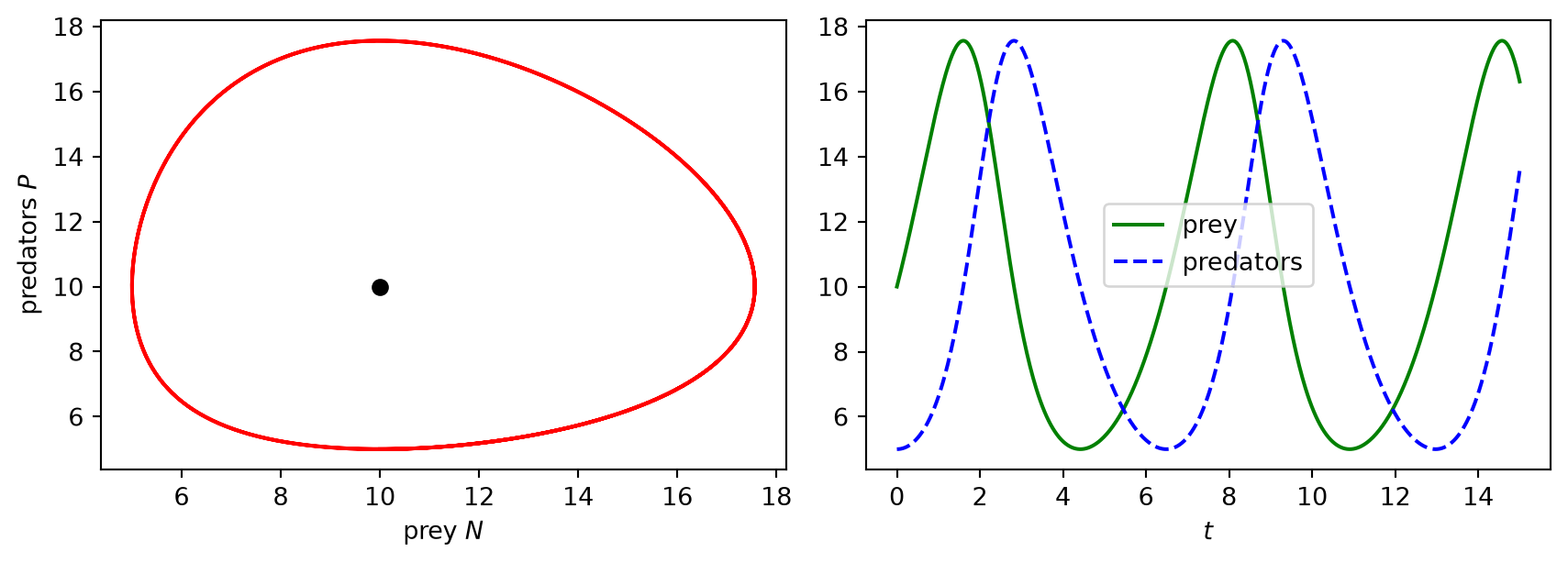
Describe the typical trajectory in the phase plane and the time series. In which order do the peaks of prey and predators occur, and why, ecologically?
Which initial condition gives no change at all? Find this steady state analytically.
What did you find about the average populations over a cycle when \(d\) was changed? Formulate a conjecture for the averages.

Explain: the average populations

Show that \(\dfrac{d}{dt}\ln P = cN-d\).
Integrate this over one period \(T\) of the oscillation. Use periodicity to show that the average \(\bar N=\frac1T\int_0^TN\,dt\) equals \(d/c\).
Similarly find the average \(\bar P\).
Suppose fishing removes both species at per-capita rate \(h\). Which parameters change and how? What happens to the average numbers of prey and predators when fishing is reduced? This answers Volterra’s question.

Check: feedback quiz 4.1

You will be asked to find steady states of predator–prey models, interpret their terms, and use the averaging argument.

Consolidation: Lotka–Volterra dynamics

The model has the steady states \((0,0)\) and \((N^*,P^*)=(d/c,\,a/b)\). All other solutions with positive initial conditions are periodic: closed loops around \((N^*,P^*)\) traversed anticlockwise, whose size depends on the initial condition. Prey peak first: when prey are abundant, predators increase. The predators then deplete the prey, and so decline themselves, after which the prey recover.

Averaged over a cycle, the populations equal their steady-state values: \(\bar N=d/c\) and \(\bar P=a/b\). Fishing both species at rate \(h\) replaces \(a\) by \(a-h\) and \(d\) by \(d+h\), so it raises the average prey population and lowers the average predator population. Reduced fishing during the war therefore favoured the predators (Volterra’s principle). The same principle explains why broad-spectrum insecticides can increase pest populations by killing their natural enemies.

Figure 4.1: A Lotka–Volterra cycle with \(a=1\), \(b=0.1\), \(c=0.1\), \(d=1\): phase plane (left) and time series (right).

4.2 Non-dimensionalisation and a conserved quantity

The model Eq. 4.2 has four parameters, but we can reduce this number by measuring \(N\), \(P\) and \(t\) in suitable units. This is called non-dimensionalisation.

Explain: non-dimensionalisation

Introduce \(u=cN/d\), \(v=bP/a\) and \(\tau=at\). Show that \[\frac{du}{d\tau}=u(1-v), \qquad \frac{dv}{d\tau}=\alpha v(u-1), \qquad \alpha=\frac da. \tag{4.3}\]
How many parameters are left? Why is \(\alpha\) dimensionless? What is the steady state now?
Why is it natural to measure \(N\) in units of its steady-state value?

Explain: the conserved quantity

Along a trajectory we can view \(v\) as a function of \(u\). Show that \(\dfrac{dv}{du}=\dfrac{\alpha v(u-1)}{u(1-v)}\).
Separate variables and integrate to show that \[H(u,v)=v-\ln v+\alpha(u-\ln u)\] is constant along trajectories.
Show that \(H\) has a minimum at \((1,1)\). Explain why the level curves of \(H\) near \((1,1)\) are closed curves, and hence why solutions are periodic.

Explore: notebook part B

Check numerically that \(H\) stays constant along a solution. Compare the trajectory with the contour lines of \(H\).
For small oscillations around \((1,1)\) the notebook measures the period. How does the period depend on \(\alpha\)? Try \(\alpha=0.25, 1, 4\) and guess a formula.
In the second cell, the prey have a small amount of self-limitation: \(du/d\tau=u(1-v-\varepsilon u)\). What happens to the cycles, even for very small \(\varepsilon\)? What happens for \(\varepsilon<0\)?

Check: feedback quiz 4.2

You will be asked to non-dimensionalise two-species models and to find conserved quantities by separating variables in \(dv/du\).

Consolidation: conserved quantity and fragility of the cycles

The non-dimensional model Eq. 4.3 has the single parameter \(\alpha=d/a\) and the steady state \((1,1)\). The quantity \(H(u,v)=v-\ln v+\alpha(u-\ln u)\) is conserved. It has a strict minimum at \((1,1)\), so orbits are closed level curves of \(H\), and every solution is periodic with an amplitude set by the initial condition. (With \(q=\ln v\), \(p=\ln u\) the equations are even Hamilton’s equations for \(H\).)

Such a conserved quantity is very special. Adding even a small extra term, such as prey self-limitation, destroys it: the orbits then spiral into the steady state, or out of it if the term has the opposite sign. We say the model is structurally unstable. We should not expect the neutral Lotka–Volterra cycles in nature. Real predator–prey cycles, such as those of lynx and snowshoe hare, need a more robust explanation (Section 4.4).

4.3 Linear stability in two dimensions

To understand behaviour near a steady state \((x^*,y^*)\) of Eq. 4.1 we linearise. Writing \(X=x^*+x\), \(Y=y^*+y\) and Taylor expanding to first order gives \[ \frac{d}{dt}\begin{pmatrix}x\\y\end{pmatrix}=A\begin{pmatrix}x\\y\end{pmatrix}, \qquad A=\begin{pmatrix}f_X & f_Y\\ g_X & g_Y\end{pmatrix}_{(x^*,y^*)}. \tag{4.4}\] \(A\) is the Jacobian matrix (in ecology also called the community matrix). So we need to understand linear systems.

Explore: notebook part C

Part C draws the phase portrait of \(\frac{d}{dt}\mathbf x=A\mathbf x\) for a matrix \(A\) that you choose with sliders. It also shows where \(A\) sits in the plane whose axes are \(\operatorname{tr}A\) and \(\det A\), and prints the eigenvalues.

Find matrices that give: trajectories all moving straight into the origin; spirals into the origin; spirals out; trajectories that come in along one direction and go out along another; closed loops.
For each, note the eigenvalues, the trace and the determinant.

Group task: the trace–determinant map

Draw large axes for \(\operatorname{tr}A\) (horizontal) and \(\det A\) (vertical) on a sheet of paper. Pool your examples and mark each with a symbol for its type (stable node, unstable node, stable spiral, unstable spiral, saddle, centre).

Find the curves in the trace–determinant plane that separate the regions. Explain them using \(\lambda^2-\operatorname{tr}(A)\lambda+\det A=0\).
Why is a saddle always unstable? What is the sign of its determinant?
What is special about points on the positive \(\det\) axis?

Explain: the Lotka–Volterra steady states

Compute the Jacobian of Eq. 4.3 at \((u,v)\).
Evaluate it at \((0,0)\) and classify this steady state.
Evaluate it at \((1,1)\). Show that the eigenvalues are \(\pm i\sqrt\alpha\). What does linearisation predict? Compare with your measured periods.
Linearisation predicts a centre at \((1,1)\). Why can we not conclude from linearisation alone that the orbits of the non-linear model are closed? What extra information did we use?

Check: feedback quiz 4.3

You will be asked to compute Jacobian matrices of two-dimensional models at steady states, compute trace, determinant and eigenvalues, and classify the steady states.

Consolidation: classification of steady states

Solutions of \(\dot{\mathbf x}=A\mathbf x\) are combinations of \(\mathbf ve^{\lambda t}\) with \(A\mathbf v=\lambda\mathbf v\). The eigenvalues are the roots of \(\lambda^2-\operatorname{tr}(A)\lambda+\det A=0\): \[ \lambda_\pm=\frac{\operatorname{tr}A\pm\sqrt{(\operatorname{tr}A)^2-4\det A}}{2}, \qquad \lambda_++\lambda_-=\operatorname{tr}A,\quad \lambda_+\lambda_-=\det A. \]

condition	eigenvalues	type
\(\det A<0\)	real, opposite signs	saddle (unstable)
\(\det A>0\), \(\operatorname{tr}A<0\), \((\operatorname{tr}A)^2\geq4\det A\)	real, both negative	stable node
\(\det A>0\), \(\operatorname{tr}A<0\), \((\operatorname{tr}A)^2<4\det A\)	complex, negative real part	stable spiral
\(\det A>0\), \(\operatorname{tr}A>0\)	positive real parts	unstable node or spiral
\(\det A>0\), \(\operatorname{tr}A=0\)	purely imaginary	centre (linear)

A steady state is stable if and only if \(\operatorname{tr}A<0\) and \(\det A>0\). Linearisation correctly predicts the behaviour of the non-linear system near the steady state whenever no eigenvalue has zero real part. For a linear centre the non-linear terms decide.

For Lotka–Volterra, \(A(u,v)=\begin{pmatrix}1-v&-u\\ \alpha v&\alpha(u-1)\end{pmatrix}\). At \((0,0)\) the eigenvalues are \(1\) and \(-\alpha\): a saddle. At \((1,1)\), \(A=\begin{pmatrix}0&-1\\ \alpha&0\end{pmatrix}\) with eigenvalues \(\pm i\sqrt\alpha\): a linear centre. Small oscillations have period \(2\pi/\sqrt\alpha\) in \(\tau\), i.e. \(2\pi/\sqrt{ad}\) in \(t\). That the non-linear orbits are closed follows from the conserved quantity \(H\), not from linearisation.

4.4 More realistic predator–prey models

A general predator–prey model has the form \[ \frac{dN}{dt}=NF(N,P), \qquad \frac{dP}{dt}=PG(N,P). \] With logistic prey growth and predation, \(F(N,P)=r(1-N/K)-R(N)P\), where \(NR(N)\) is the rate at which one predator eats prey, called the functional response. Holling distinguished three types:

Type I, \(NR(N)=bN\): consumption increases without limit (Lotka–Volterra).
Type II, \(NR(N)=\dfrac{AN}{N+B}\): consumption saturates at \(A\), because each prey item takes time to handle.
Type III, \(NR(N)=\dfrac{AN^2}{N^2+B^2}\): like type II, but predators rarely catch scarce prey (for example because they switch to other prey or have to learn to hunt it).

Predict

Sketch the three functional responses. Which one do you think best describes a fox eating rabbits? A whale filtering plankton?

We study the model with a Holling type II response in which the predators’ carrying capacity is proportional to the prey abundance: \[ \frac{dN}{dt}=N\left[r\left(1-\frac NK\right)-\frac{AP}{N+B}\right], \qquad \frac{dP}{dt}=sP\left(1-\frac{hP}{N}\right). \] With \(u=N/K\), \(v=hP/K\), \(\tau=rt\), \(a=A/(hr)\), \(b=B/K\) and \(c=s/r\) it becomes \[ \frac{du}{d\tau}=u(1-u)-\frac{a\,uv}{u+b}, \qquad \frac{dv}{d\tau}=cv\left(1-\frac vu\right). \tag{4.5}\]

Explore: notebook part D

Set \(a=1\), \(b=0.1\) and vary \(c\) between \(0.05\) and \(1\). Describe the long-term behaviour. For which values of \(c\) do the populations settle down, and for which do they oscillate?
In the oscillating case, start from several different initial conditions. How is this different from Lotka–Volterra?
Find (approximately) the value of \(c\) at which the behaviour changes. What happens to the eigenvalues of the coexistence steady state there?

Explain

Show that the steady states with \(u>0\) are \((1,0)\) and \((u^*,u^*)\), with \(u^*=\frac12\left(1-a-b+\sqrt{(1-a-b)^2+4b}\right)\).
Show that \((1,0)\) is a saddle.
At \((u^*,u^*)\) show that \(g_u=c\), \(g_v=-c\) and \(f_v=-(1-u^*)\), using the steady-state condition \(1-u^*=au^*/(u^*+b)\). Deduce that \(\det A=c\left(u^*+\frac{b(1-u^*)}{u^*+b}\right)>0\).
Hence show that the coexistence state is stable if and only if \(c>f_u\), where \(f_u=1-2u^*-\frac{b(1-u^*)}{u^*+b}\). Compare with part D.

Check: feedback quiz 4.4

You will be asked to identify functional responses, non-dimensionalise a predator–prey model, and determine the stability of its steady states.

Consolidation: limit cycles

In model Eq. 4.5 the coexistence steady state always has \(\det A>0\), so it is never a saddle. It is stable when \(c>f_u\): predators respond fast enough to damp the oscillations. When \(c<f_u\) the steady state is an unstable spiral, and the trajectories approach a limit cycle: an isolated periodic orbit that attracts all nearby trajectories. Unlike the Lotka–Volterra cycles, its amplitude and period do not depend on the initial condition, and it survives small changes to the model. Limit cycles are therefore a robust explanation for population cycles observed in nature. The change at \(c=f_u\), where a pair of complex eigenvalues crosses the imaginary axis and a limit cycle is born, is a Hopf bifurcation. By the Poincaré–Bendixson theorem, a bounded trajectory in the plane that approaches no steady state must approach a periodic orbit.

4.5 Exam-style questions

Exam-style question 4.1: classification

Classify the steady state at the origin of \(\dot{\mathbf x}=A\mathbf x\) for \[ \text{(a) } A=\begin{pmatrix}-1&2\\-3&1\end{pmatrix},\qquad \text{(b) } A=\begin{pmatrix}2&1\\3&-1\end{pmatrix},\qquad \text{(c) } A=\begin{pmatrix}-3&1\\1&-2\end{pmatrix}. \] [6 marks]

Solution

\(\operatorname{tr}=0\), \(\det=-1+6=5>0\): a centre (eigenvalues \(\pm i\sqrt5\)).
\(\det=-2-3=-5<0\): a saddle.
\(\operatorname{tr}=-5\), \(\det=6-1=5>0\), \(\operatorname{tr}^2-4\det=5>0\): a stable node.

Exam-style question 4.2: a predator with a saturating response

A model for two interacting species is \[ \frac{dN_1}{dt}=rN_1\left(1-\frac{N_1}{K}\right)-aN_1N_2\left(1-e^{-bN_1}\right),\qquad \frac{dN_2}{dt}=-dN_2+cN_2\left(1-e^{-bN_1}\right), \] with positive constants \(a,b,c,d,r,K\).

With \(u=N_1/K\), \(v=aN_2/r\), \(\tau=rt\) and \(\beta=bK\) show that \[ \frac{du}{d\tau}=u(1-u)-uv\left(1-e^{-\beta u}\right),\qquad \frac{dv}{d\tau}=-\delta v+\alpha v\left(1-e^{-\beta u}\right), \] and give \(\alpha\) and \(\delta\). [3 marks]
Describe the relevance of each term. What type of interaction is this? [3 marks]
Show that the non-negative steady states are \((0,0)\), \((1,0)\) and \((u_1,(1-u_1)\alpha/\delta)\) with \(u_1=-\ln(1-\delta/\alpha)/\beta\), and that the last exists only if \(\alpha>\delta\) and \(\beta>\beta_c=-\ln(1-\delta/\alpha)\). [4 marks]
Assuming \(\alpha>\delta\), determine the stability of each steady state. [6 marks]

Solution

\(\frac{du}{d\tau}=\frac{1}{rK}\frac{dN_1}{dt}\) gives the first equation, and \(\frac{dv}{d\tau}=\frac{a}{r^2}\frac{dN_2}{dt}\) gives the second with \(\delta=d/r\) and \(\alpha=c/r\).
\(u(1-u)\): logistic growth of species 1. \(-uv(1-e^{-\beta u})\): predation, with a functional response that saturates at high prey density (similar to Holling type II). \(-\delta v\): predator mortality. \(\alpha v(1-e^{-\beta u})\): predator reproduction from eating prey. This is a predator–prey interaction, with species 2 the predator.
\(dv/d\tau=0\) with \(v\neq0\) requires \(1-e^{-\beta u}=\delta/\alpha\), which needs \(\alpha>\delta\) and gives \(u_1\). Then \(du/d\tau=0\) with \(u\neq0\) gives \(1-u=v\delta/\alpha\), so \(v=(1-u_1)\alpha/\delta\), positive iff \(u_1<1\), iff \(\beta>\beta_c\).
The Jacobian is \(A=\begin{pmatrix}1-2u-v(1-e^{-\beta u})-\beta uve^{-\beta u}&-u(1-e^{-\beta u})\\ \alpha\beta ve^{-\beta u}&-\delta+\alpha(1-e^{-\beta u})\end{pmatrix}\).

At \((0,0)\) the eigenvalues are \(1\) and \(-\delta\): a saddle.
At \((1,0)\) the eigenvalues are \(-1\) and \(\alpha(1-e^{-\beta})-\delta\), which is positive iff \(\beta>\beta_c\). So \((1,0)\) is a saddle if \(\beta>\beta_c\) and a stable node if \(\beta<\beta_c\).
At the coexistence state \(A_{22}=0\) and \(A_{12}A_{21}<0\), so \(\det A>0\). Using \(1-u_1=v(1-e^{-\beta u_1})\), \(\operatorname{tr}A=A_{11}=-u_1-\beta u_1ve^{-\beta u_1}<0\). So the coexistence state is stable (a node or a spiral).

Exam-style question 4.3: predator–prey with an Allee effect

Consider \[ \frac{dN}{dT}=rN\left(\frac N{K_0}-1\right)\left(1-\frac NK\right)-cNP,\qquad \frac{dP}{dT}=bNP-mP, \] with positive constants and \(0<K_0<K\).

Interpret the parameters. What is the role of \(K_0\)? [3 marks]
With \(x=N/K\), \(y=cP/r\), \(t=rT\) show that \[\frac{dx}{dt}=x\,(g(x)-y),\qquad \frac{dy}{dt}=\beta(x-\alpha)y,\qquad g(x)=\left(\frac x\gamma-1\right)(1-x),\] and express \(\alpha,\beta,\gamma\) in terms of the original parameters. [3 marks]
Find the nullclines and the steady states, and sketch the nullclines. [4 marks]
For \(\gamma<\alpha<1\) find the Jacobian at the coexistence steady state in terms of \(g\) and \(g'\) and classify the steady state as \(\alpha\) varies. [6 marks]

Solution

\(r\): prey growth rate scale. \(K\): prey carrying capacity. \(K_0\): Allee threshold, below which the prey decline even without predators. \(c\): predation rate per predator. \(b\): predator reproduction per prey eaten per unit time. \(m\): predator mortality rate.
\(\gamma=K_0/K\), \(\beta=bK/r\), \(\alpha=m/(bK)\).
\(x\)-nullclines: \(x=0\) and \(y=g(x)\), a downward parabola with zeros at \(\gamma\) and \(1\). \(y\)-nullclines: \(y=0\) and \(x=\alpha\). Steady states: \((0,0)\), \((\gamma,0)\), \((1,0)\) and \((\alpha,g(\alpha))\), which is positive for \(\gamma<\alpha<1\).
\(A=\begin{pmatrix}g(x)-y+xg'(x)&-x\\ \beta y&\beta(x-\alpha)\end{pmatrix}\), so at \((\alpha,g(\alpha))\), \(A=\begin{pmatrix}\alpha g'(\alpha)&-\alpha\\ \beta g(\alpha)&0\end{pmatrix}\). Then \(\det A=\alpha\beta g(\alpha)>0\) and \(\operatorname{tr}A=\alpha g'(\alpha)\), with \(g'(x)=(1+\gamma-2x)/\gamma\). So:

\(\gamma<\alpha<\frac{1+\gamma}2\): \(\operatorname{tr}>0\), unstable (spiral if \(\operatorname{tr}^2<4\det\), otherwise node);
\(\alpha=\frac{1+\gamma}2\): linear centre (Hopf bifurcation point);
\(\frac{1+\gamma}2<\alpha<1\): \(\operatorname{tr}<0\), stable (spiral or node).

Summary

Lotka–Volterra: \(\dot N=N(a-bP)\), \(\dot P=P(cN-d)\). It has neutral cycles around \((d/c,a/b)\), a conserved quantity \(H\), and averages equal to the steady state (Volterra’s principle). The cycles are structurally unstable.
Non-dimensionalisation reduces the number of parameters and reveals which combinations matter.
Linear stability: compute the Jacobian at the steady state. The state is stable iff \(\operatorname{tr}A<0\) and \(\det A>0\). \(\det A<0\) means a saddle, and complex eigenvalues mean a spiral.
Functional responses (Holling types I–III) describe how predator consumption depends on prey density. Realistic models can have stable steady states or limit cycles, which are born in Hopf bifurcations.

4.6 Launch: competing species

Launch investigation for week 5

Open the week 5 notebook in Colab

In the 1930s the Russian biologist G. F. Gause grew two species of Paramecium separately and together. Alone, each species settled at a stable population. Together, one of them always died out. We use the Lotka–Volterra competition model, written in non-dimensional form: \[ \frac{du_1}{d\tau}=u_1(1-u_1-a_{12}u_2),\qquad \frac{du_2}{d\tau}=\rho u_2(1-u_2-a_{21}u_1). \]

Before running anything: what does \(a_{12}\) measure? What would you expect if both \(a_{12}\) and \(a_{21}\) are small? If both are large?
In part A of the notebook, explore the \((a_{12},a_{21})\) parameter space. Find four qualitatively different outcomes. For each, note the parameter values and sketch the phase portrait.
Draw the square \(0\le a_{12}\le2\), \(0\le a_{21}\le2\) and divide it into regions according to the outcome. Can you guess where the boundaries are?
Does \(\rho\) affect the outcome?