3 Discrete-time models
Many species breed once a year: fish spawn in spring, birds breed in summer, annual plants set seed and die in the winter. Instead of following the population continuously through time, it is then natural to follow it from one year to the next, \[ N_{t+1}=f(N_t), \qquad t=0,1,2,\ldots \tag{3.1}\] Given \(N_0\), iterating the map gives \(N_1=f(N_0)\), \(N_2=f(f(N_0))\), and so on. In the launch investigation you saw that such models can behave very differently from their continuous-time cousins.
TipLearning outcomes for this week
By the end of this week you should be able to:
- formulate discrete-time population models and interpret their parameters;
- find fixed points of maps and determine their stability by linearisation;
- draw and interpret cobweb diagrams;
- analyse the Verhulst, Ricker and Beverton–Holt models;
- explain what a period-doubling bifurcation is and describe the route to chaos;
- solve the Beverton–Holt model exactly.
Open the week 3 notebook in Colab
3.1 From annual breeding to maps
The simplest discrete-time model is \(N_{t+1}=RN_t\), with solution \(N_t=N_0R^t\). Here \(R>0\) is a dimensionless growth factor, not a rate. The population grows if \(R>1\) and declines if \(R<1\).
NoteExplain: growth rates and growth factors
- Show that \(N_t=N_0R^t\) agrees with the continuous-time solution \(N(t)=N_0e^{rt}\) at integer times if \(R=e^{r\cdot 1\,\text{year}}\).
- A savings account quotes an annual equivalent rate (AER) of 5%, i.e. \(R=1.05\). What is the corresponding continuous interest rate \(r\)?
In the launch investigation you explored the Verhulst model \[ N_{t+1}=N_t+R_0N_t\left(1-\frac{N_t}{K}\right) = RN_t\left(1-\frac{N_t}{\tilde K}\right), \tag{3.2}\] with \(R=1+R_0\) and \(\tilde K=K(1+R_0)/R_0\). The first form shows that the population changes each year by an amount given by the logistic expression. The second form shows that the map is a parabola. It is also known as the logistic map and is one of the most famous examples of chaos.
WarningGroup task: pooling the launch results
Compare your descriptions of the time series from the launch investigation.
- Agree on the ranges of \(R_0\) for which the population (a) approaches \(K\) monotonically, (b) approaches \(K\) with damped oscillations, (c) settles into an oscillation between two values, (d) does something more complicated.
- Describe ecologically what is happening when the population overshoots \(K\).
- Why can the continuous-time logistic model never oscillate?
A fixed point of the map is a value \(N^*\) with \(f(N^*)=N^*\): a population size that stays the same from year to year. For the Verhulst model the fixed points are \(N^*=0\) and \(N^*=K\).
NoteCheck: feedback quiz 3.1
You will be asked to find fixed points of given maps and to convert between growth rates and growth factors.
3.2 Cobweb diagrams and stability
TipExplore: notebook part B
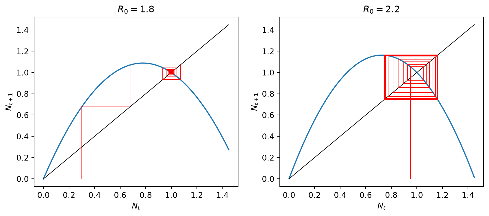
A cobweb diagram shows how the sequence \(N_t\) is generated. Start at \(N_0\) on the horizontal axis, go vertically to the graph of \(f\) to find \(N_1\), then horizontally to the diagonal \(N_{t+1}=N_t\) so that \(N_1\) becomes the new input, then vertically to the graph again, and so on.
- Use part B to draw cobwebs for the Verhulst model with \(R_0=0.5\), \(1.5\) and \(2.5\). Where are the fixed points in the cobweb diagram?
- Relate the shape of the cobweb (staircase or spiral, inwards or outwards) to the slope of \(f\) at the fixed point.
- In the second cell of part B you can enter your own map. The notebook prints \(f'(N^*)\) at each fixed point. Formulate a conjecture for when a fixed point is stable. Test it on at least three maps.
NoteExplain: linear stability of fixed points
- Write \(N_t=N^*+n_t\) with \(n_t\) small and Taylor expand to show \(n_{t+1}\approx f'(N^*)\,n_t\).
- Solve this linear recurrence and deduce the stability criterion. When does \(n_t\) change sign every year?
- Compare with the criterion for continuous-time models. Why is it different?
- Apply the criterion to the Verhulst model: for which \(R_0>0\) is \(N^*=K\) stable?
NoteCheck: feedback quiz 3.2
You will be asked to compute \(f'(N^*)\) for given maps, classify the fixed points (stable or unstable, monotonic or oscillatory approach), and find parameter ranges for stability.
NoteConsolidation: stability of fixed points of maps
Near a fixed point, \(n_{t+1}\approx f'(N^*)n_t\), so \(n_t\approx n_0\,(f'(N^*))^t\).
- If \(|f'(N^*)|<1\) the fixed point is stable. If \(|f'(N^*)|>1\) it is unstable. If \(|f'(N^*)|=1\) linearisation is inconclusive.
- If \(f'(N^*)>0\) the perturbation keeps its sign, and the cobweb is a staircase. If \(f'(N^*)<0\) the population alternates above and below \(N^*\), and the cobweb is a spiral.
For the Verhulst model \(f'(N)=1+R_0(1-2N/K)\), so \(f'(0)=1+R_0\) and \(f'(K)=1-R_0\). The fixed point \(K\) is stable for \(0<R_0<2\), approached monotonically for \(R_0<1\) and with damped oscillations for \(1<R_0<2\). Ecologically, a large growth factor makes the population overshoot the carrying capacity in one breeding season, so that conditions are poor the following year. A continuous-time single-species model cannot oscillate, because solutions cannot jump over a steady state.
WarningGroup task: negative populations
For some parameter values the Verhulst model predicts negative population numbers, even when it starts with a positive population. Find the condition on \(R\) (in the form \(N_{t+1}=RN_t(1-N_t/\tilde K)\)) under which this can happen. Hint: think about what the cobweb diagram would have to look like.
NoteConsolidation: negative populations
The map \(f(N)=RN(1-N/\tilde K)\) is negative for \(N>\tilde K\). A population between \(0\) and \(\tilde K\) can be mapped above \(\tilde K\) if the maximum of \(f\), which is \(f(\tilde K/2)=R\tilde K/4\), exceeds \(\tilde K\). So for \(R>4\) (equivalently \(R_0>3\)) a population starting near \(\tilde K/2\) jumps above \(\tilde K\) in one year and becomes negative the year after. For \(R\leq4\) the map sends \([0,\tilde K]\) into itself and populations stay non-negative.
3.3 The Ricker and Beverton–Holt models
Because the Verhulst model can produce negative numbers, fisheries scientists use other maps. Ricker introduced his model to describe salmon, whose spawning success drops sharply at high density: \[ N_{t+1}=N_te^{R_0(1-N_t/K)}. \tag{3.3}\] Beverton and Holt, working at the Fisheries Laboratory in Lowestoft in the 1950s, proposed \[ N_{t+1}=\frac{RN_t}{1+\frac{R-1}{K}N_t}. \tag{3.4}\]
NotePredict
Look at the shapes of the two maps in part C of the notebook, with the sliders at their default values. Before experimenting, predict which of the two models can produce oscillations.
TipExplore: notebook part C
- For each model, find the fixed points and their stability from the notebook, for a range of parameter values.
- For the Ricker model find (numerically) the value of \(R_0\) at which the fixed point \(K\) loses stability. What happens to the population beyond it?
- Can you make the Beverton–Holt model oscillate?
NoteExplain
- Show that both models have fixed points \(0\) and \(K\).
- Compute \(f'(0)\) and \(f'(K)\) for each model. Determine the stability of the fixed points. For the Ricker model allow negative \(R_0\) too: how many bifurcations do you find?
- Show that the Beverton–Holt map is increasing, and explain why this means its solutions cannot oscillate.
WarningGroup task: solving the Beverton–Holt model
The Beverton–Holt model can be solved exactly.
- Write \(u_t=1/N_t\) and show that \(u_{t+1}=\dfrac{u_t}{R}+\dfrac{R-1}{RK}\). This is a linear recurrence.
- Find its fixed point \(u^*\) and show that \(u_t-u^*\) satisfies a recurrence you can solve.
- Hence show that \[N_t=\frac{KN_0}{N_0+(K-N_0)R^{-t}}.\]
- Compare this with the solution Eq. 1.4 of the continuous logistic model. What is the relation between \(R\) and \(r\)?
NoteCheck: feedback quiz 3.3
You will be asked to find and classify the fixed points of Ricker- and Beverton–Holt-type maps and to find the parameter values at which they change stability.
NoteConsolidation: Ricker and Beverton–Holt
Ricker. \(f'(N)=(1-R_0N/K)e^{R_0(1-N/K)}\), so \(f'(0)=e^{R_0}\) and \(f'(K)=1-R_0\). The extinction state is stable for \(R_0<0\) and unstable for \(R_0>0\). The fixed point \(K\) is stable for \(0<R_0<2\). There are two bifurcations: at \(R_0=0\), where \(f'(K)=1\) and \(0\) and \(K\) exchange stability (transcritical), and at \(R_0=2\), where \(f'(K)=-1\) and \(K\) loses stability in a period-doubling bifurcation. Like the Verhulst model, the Ricker model can oscillate and becomes chaotic for larger \(R_0\), but \(N_t\) always stays positive.
Beverton–Holt. \(f'(N)=R\big/\left(1+\frac{R-1}{K}N\right)^2>0\), with \(f'(0)=R\) and \(f'(K)=1/R\). For \(R>1\) the fixed point \(K\) is stable and approached monotonically. With \(u_t=1/N_t\) the model becomes linear, and its solution \[ N_t=\frac{KN_0}{N_0+(K-N_0)R^{-t}} \] coincides at integer times with the logistic solution if \(R=e^{r}\). The Beverton–Holt model is therefore the exact discrete-time counterpart of the logistic model. In fisheries it describes how the number of young fish (recruits) depends on the spawning stock.
3.4 Period doubling and chaos
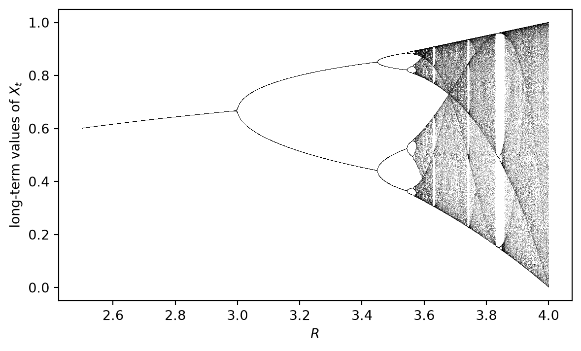
What happens to the Verhulst model beyond \(R_0=2\)? It is convenient to rescale \(X_t=N_t/\tilde K\) and study the logistic map \(X_{t+1}=RX_t(1-X_t)\) with \(R=1+R_0\), so that the fixed point \(1-1/R\) loses stability at \(R=3\).
TipExplore: notebook part D
- The orbit diagram shows, for each \(R\), the values the population keeps visiting after a long time. Describe what happens as \(R\) increases from \(2.5\) to \(4\). Zoom in using the sliders.
- Estimate the values of \(R\) at which the period doubles from 1 to 2, from 2 to 4 and from 4 to 8. What do you notice about the gaps between them?
- For \(R=3.9\), start two populations that differ by \(10^{-6}\). How long does it take before their time series look completely different? Why is this important for prediction?
NoteExplain: the period-2 orbit
A period-2 orbit consists of two values \(x_1\neq x_2\) with \(f(x_1)=x_2\) and \(f(x_2)=x_1\). They are fixed points of the composed map \(f\circ f\).
- By the chain rule, \((f\circ f)'(x_1)=f'(x_2)f'(x_1)\). Explain why the period-2 orbit is stable if \(|f'(x_1)f'(x_2)|<1\).
- Explain why a period-2 orbit appears when \(f'(N^*)\) passes through \(-1\). (Think about the cobweb.)
NoteCheck: feedback quiz 3.4
You will be asked to find parameter values at which period-doubling bifurcations occur and to identify types of bifurcation from the value of \(f'(N^*)\).
NoteConsolidation: bifurcations of maps and the route to chaos
Fixed points of maps change stability when \(|f'(N^*)|\) passes through \(1\).
- \(f'(N^*)=1\): the same bifurcations as for ODEs, i.e. saddle-node (tangent), transcritical and pitchfork.
- \(f'(N^*)=-1\): a period-doubling bifurcation. The fixed point becomes unstable and a stable period-2 orbit is born around it. This bifurcation is impossible for one-dimensional ODEs.
In the logistic map the fixed point loses stability at \(R=3\). The period-2 orbit \(x_{1,2}=\left(R+1\pm\sqrt{(R+1)(R-3)}\right)/(2R)\) is stable up to \(R=1+\sqrt6\approx3.449\), where it period-doubles to a period-4 orbit, and so on. The bifurcation values accumulate at \(R\approx3.5699\), beyond which the dynamics are mostly chaotic, with windows of periodic behaviour. The ratio of successive gaps between period doublings tends to the Feigenbaum constant \(4.669\ldots\), the same for all smooth one-humped maps.
Chaotic dynamics show sensitive dependence on initial conditions: tiny differences grow exponentially, so long-term prediction is impossible even though the model is deterministic. How important chaos is in real ecological systems is still debated. A famous paper by May (May 1976) alerted biologists to these possibilities.
3.5 Exam-style questions
ImportantExam-style question 3.1: Ricker model
Find the fixed points of the Ricker model Eq. 3.3, with \(K>0\) and \(R_0\in\mathbb R\), and investigate their stability. Illustrate your results with cobweb diagrams: you will need one for each of the three parameter regions separated by the two bifurcations. [8 marks]
NoteSolution
Fixed points: \(N=Ne^{R_0(1-N/K)}\) gives \(N^*=0\) or \(e^{R_0(1-N/K)}=1\), i.e. \(N^*=K\). \(f'(N)=e^{R_0(1-N/K)}(1-R_0N/K)\), so \(f'(0)=e^{R_0}\) and \(f'(K)=1-R_0\).
- \(R_0<0\): \(0\) is stable (\(0<f'(0)<1\)) and \(K\) is unstable (\(f'(K)>1\)). The cobweb shows staircases away from \(K\) towards \(0\) (for \(N_0<K\)) and towards infinity (for \(N_0>K\)).
- \(0<R_0<2\): \(0\) is unstable and \(K\) is stable. The approach is monotonic for \(R_0<1\) (staircase) and oscillatory for \(1<R_0<2\) (inward spiral).
- \(R_0>2\): both are unstable. The cobweb spirals outward from \(K\) towards a period-2 orbit (and for larger \(R_0\) more complex behaviour).
Bifurcations: transcritical at \(R_0=0\) and period-doubling at \(R_0=2\).
ImportantExam-style question 3.2: Beverton–Holt model
Find the fixed points of the Beverton–Holt model Eq. 3.4 with \(R>0\), \(K>0\) and determine their stability. Sketch cobweb diagrams for \(R>1\) and \(0<R<1\). [6 marks]
NoteSolution
\(N=\frac{RN}{1+(R-1)N/K}\) gives \(N=0\) or \(1+(R-1)N/K=R\), i.e. \(N=K\). Also \(f'(N)=\frac{R}{(1+(R-1)N/K)^2}\), so \(f'(0)=R\) and \(f'(K)=1/R\). For \(R>1\), \(0\) is unstable and \(K\) is stable. For \(R<1\), \(0\) is stable and \(K\) is unstable. Since \(f'>0\), all cobwebs are staircases: for \(R>1\) they climb towards \(K\) from below (or descend from above). There is a transcritical bifurcation at \(R=1\).
ImportantExam-style question 3.3: period-doubling bifurcation
Consider the model \[ N_{t+1}=\frac{rN_t}{1+(N_t/K)^b} \] with positive parameters \(r\), \(K\) and \(b>1\).
Show that for \(r>1\) there are two non-negative fixed points and investigate the stability of the extinction state. [3 marks]
Show that the non-trivial fixed point loses stability through a period-doubling bifurcation at \(b=2r/(r-1)\). [5 marks]
What happens to the non-trivial fixed point as \(r\) decreases to \(1\)? [2 marks]
NoteSolution
\(N^*=0\) or \(1+(N^*/K)^b=r\), i.e. \(N^*=K(r-1)^{1/b}\), which is positive for \(r>1\). Since \(f'(0)=r\), the extinction state is unstable for \(r>1\) and stable for \(r<1\).
\(f'(N)=\dfrac{r}{1+(N/K)^b}-\dfrac{rb(N/K)^b}{(1+(N/K)^b)^2}\). At \(N^*\), \(1+(N^*/K)^b=r\) and \((N^*/K)^b=r-1\), so \(f'(N^*)=1-\dfrac{b(r-1)}{r}\). This is less than \(1\). It equals \(-1\) when \(b(r-1)/r=2\), i.e. \(b=2r/(r-1)\), and for larger \(b\) we have \(f'(N^*)<-1\). So the fixed point loses stability through a period-doubling bifurcation.
As \(r\to1^+\), \(N^*\to0\) and \(f'(N^*)\to1\). The non-trivial fixed point merges with the extinction state, which becomes stable for \(r<1\) (the bifurcation has \(f'=1\)).
ImportantExam-style question 3.4: harvesting with depensation
A population follows \(N_{t+1}=f(N_t)\) with \[ f(N)=\frac{bN^2}{1+N^2}-EN, \] where \(b>2\) and \(E\geq0\) is the harvesting effort.
For \(E=0\), find the fixed points and determine their stability. Sketch the graph of \(f\) together with the diagonal. [5 marks]
Find the critical effort \(E_c\) above which the population goes extinct from any initial condition. What type of bifurcation occurs at \(E_c\)? [4 marks]
NoteSolution
\(N^*=0\) or \(1+N^2=bN\), i.e. \(N^*_\pm=\frac{b\pm\sqrt{b^2-4}}2\). The graph of \(f\) behaves like \(bN^2\) near \(0\) (so \(f'(0)=0\) and \(0\) is stable), is increasing, and tends to \(b\) as \(N\to\infty\). It crosses the diagonal at \(N^*_-\) from below (slope \(>1\), unstable) and at \(N^*_+\) from above (slope \(<1\), stable). \(N^*_-\) is the minimum viable population: critical depensation.
Non-zero fixed points satisfy \((1+E)N^2-bN+(1+E)=0\), so \(N^*_\pm=\frac{1}{2}\left(\frac{b}{1+E}\pm\sqrt{\left(\frac{b}{1+E}\right)^2-4}\right)\). They exist while \(b/(1+E)\geq2\), i.e. \(E\leq E_c=\frac{b-2}{2}\). At \(E_c\) the two fixed points merge and disappear in a saddle-node (tangent) bifurcation.
ImportantExam-style question 3.5 (longer): house finches
This question combines continuous dynamics within a year (time \(\tau\)) with a discrete map from year to year (year \(t\)).
At the start of winter, house finches (combined number \(N_t\), sex ratio 1:1) search for mates for a time \(T\). Unpaired males \(M\) and females \(F\) meet at random and form pairs at rate \(\sigma MF\), so that \(dM/d\tau=dF/d\tau=-\sigma MF\). A fraction \(G(P)=1/(1+P/\delta)\) of the \(P\) pairs find a nest site and breed, producing \(c\) offspring each. Each bird survives to the next year with probability \(s\).
Show that the number \(n=M+F\) of unpaired birds satisfies \(dn/d\tau=-\frac\sigma2n^2\) with \(n(0)=N_t\), and that \(n(T)=rN_t/(r+2N_t)\) with \(r=4/(\sigma T)\). [4 marks]
Explain why the number of pairs satisfies \(dP/d\tau=-\frac12dn/d\tau\), and show that \(P_t=P(T)=N_t^2/(r+2N_t)\). [3 marks]
Show that \[N_{t+1}=sN_t+\frac{cN_t^2}{r+2N_t+N_t^2/\delta}.\] [2 marks]
Find the positive fixed points when \(\frac{c}{1-s}-2\geq\sqrt{4r/\delta}\). Draw a cobweb diagram showing their stability when there are two of them. What bifurcation occurs when equality holds? [6 marks]
NoteSolution
With \(M=F=n/2\): \(dn/d\tau=-2\sigma MF=-\frac\sigma2n^2\). Separating, \(\frac1{n(T)}-\frac1{N_t}=\frac{\sigma T}{2}=\frac2r\), so \(n(T)=\frac{N_t}{1+2N_t/r}=\frac{rN_t}{r+2N_t}\).
Each new pair removes two unpaired birds, so \(dP/d\tau=-\frac12dn/d\tau\). Integrating from \(P(0)=0\): \(P(T)=\frac12(N_t-n(T))=\frac{N_t}2\cdot\frac{2N_t}{r+2N_t}=\frac{N_t^2}{r+2N_t}\).
\(N_{t+1}=sN_t+cG(P_t)P_t=sN_t+\frac{cP_t}{1+P_t/\delta}\). Substituting \(P_t\) and multiplying numerator and denominator by \(r+2N_t\) gives the result.
Non-zero fixed points satisfy \((1-s)(r+2N+N^2/\delta)=cN\), i.e. \(N^2/\delta-\left(\frac c{1-s}-2\right)N+r=0\), so \[N^*_\pm=\frac\delta2\left[\left(\frac{c}{1-s}-2\right)\pm\sqrt{\left(\frac{c}{1-s}-2\right)^2-\frac{4r}\delta}\right].\] These are real and positive under the stated condition. Since \(f'(0)=s<1\), \(0\) is stable. The graph of \(f\) crosses the diagonal from below at \(N^*_-\) (unstable) and from above at \(N^*_+\) (stable, assuming the slope there is greater than \(-1\)). At equality the two fixed points merge: a saddle-node (tangent) bifurcation.
Summary
- Discrete-time models \(N_{t+1}=f(N_t)\) suit populations with seasonal breeding. The growth factor \(R\) corresponds to \(e^r\).
- Fixed points satisfy \(f(N^*)=N^*\). They are stable if \(|f'(N^*)|<1\), and the approach is oscillatory if \(f'(N^*)<0\).
- Cobweb diagrams visualise iteration. Staircases correspond to positive slope and spirals to negative slope.
- Verhulst (logistic map): \(K\) is stable for \(0<R_0<2\), and the model can give negative numbers. Ricker: \(K\) is stable for \(0<R_0<2\), and numbers stay positive. Beverton–Holt: monotone, exactly solvable, the discrete counterpart of the logistic model.
- Bifurcations of maps occur at \(f'(N^*)=1\) (saddle-node, transcritical, pitchfork) or \(f'(N^*)=-1\) (period doubling). Cascades of period doublings lead to chaos.
3.6 Launch: predators and prey
NoteLaunch investigation for week 4
Open the week 4 notebook in Colab
In the 1920s the Italian mathematician Vito Volterra was asked by his future son-in-law, a marine biologist, why the proportion of predatory fish caught in the Adriatic had risen during the First World War, when fishing was reduced. Volterra (and independently Alfred Lotka) proposed the model \[ \frac{dN}{dt}=N(a-bP), \qquad \frac{dP}{dt}=P(cN-d) \] for prey \(N\) and predators \(P\).
- Before running anything: explain the meaning of each term. What do you expect to happen?
- In part A of the notebook, look at the time series and at the trajectory in the \((N,P)\) plane. Describe what you see. Which population peaks first?
- Change the initial conditions. What changes and what stays the same?
- Are there initial conditions for which nothing changes?
- Increase the predator death rate \(d\) (as would happen with more fishing of predators). What happens to the average numbers of prey and predators over a cycle? Does this help answer Volterra’s question?