Exploring the Simulation Results

Introduction

In the sections on the multispecies model and on running a simulation we saw how to set up a model and project it forward through time under our desired fishing scenario. The result of running a projection is an object of class MizerSim. What do we then do? How can we explore the results of the simulation? In this section we introduce a range of summaries, plots and indicators that can be easily produced using functions included in mizer.

We will use the same MizerSim object for these examples:

sim <- project(params_gears, effort = effort_array, dt = 0.1, t_save = 1)

Directly accessing the slots of MizerSim objects

We have seen in previous sections that a MizerSim object is made up of various slots that contain the original parameters (species_params), the population abundances (n), the abundance of the plankton spectrum (n_pp), possibly the abundances of other components (n_other), and the fishing effort (effort).

The projected species abundances at size through time can be seen in the n slot. This is a three-dimensional array (time x species x size). Consequently, this array can get very big so inspecting it can be difficult. In the example we have just run, the time dimension of the n slot has 10 rows (one for the initial population and then one for each of the saved time steps). There are also 12 species each with 100 sizes. We can check this by running the dim() function and looking at the dimensions of the n array:

dim(sim@n)

## [1]  10  12 100

To pull out the abundances of a particular species through time at size you can subset the array. For example to look at Cod through time you can use:

sim@n[, "Cod", ]

This returns a two-dimensional array: time x size, containing the cod abundances. The time dimension depends on the value of the argument t_save when project() was run. You can see that even though we specified dt to be 0.1 when we called project(), the t_save = 1 argument has meant that the output is only saved every year.

The n_pp slot can be accessed in the same way.

Summary functions

As well as the summary() methods that are available for both MizerParams and MizerSim objects, there are other useful summary functions to pull information out of a MizerSim object. A description of the different summary functions available is given in the summary functions help page.

All of these functions have help files to explain how they are used. (It is also possible to use most of these functions with a MizerParams object if you also supply the population abundance as an argument. This can be useful for exploring how changes in parameter value or abundance can affect summary statistics and indicators. We won’t explore this here but you can see their help files for more details.)

The functions getBiomass() and getN() have additional arguments that allow the user to set the size range over which to calculate the summary statistic. This is done by passing in a combination of the arguments min_l, min_w, max_l and max_w for the minimum and maximum length or weight.

If min_l is specified there is no need to specify min_w and so on. However, if a length is specified (minimum or maximum) then it is necessary for the species parameter data.frame (see the species parameters section) to include the parameters a and b for length-weight conversion. It is possible to mix length and weight constraints, e.g. by supplying a minimum weight and a maximum length. The default values are the minimum and maximum weights of the spectrum, i.e. the full range of the size spectrum is used.

Examples of using the summary functions

Here we show a simple demonstration of using a summary function using the sim object we created earlier. Here, we use getSSB() to calculate the SSB of each species through time (note the use of the head() function to only display the first few rows).

ssb <- getSSB(sim)
dim(ssb)

## [1] 10 12

head(ssb)

##     sp
## time        Sprat      Sandeel       N.pout      Herring         Dab
##    1     49711139 8.446322e+07     72985106     51266707    73542870
##    2    814017445 3.183278e+11 221192687843  11683784963 22427436185
##    3  10695137487 9.136293e+11 276051781272 289058799237 52060677753
##    4  20022819347 9.074525e+11  52552147654 232639993705 23424469977
##    5  68459460440 1.164780e+12  23794924123  83694993951 13670791573
##    6 165668862948 1.571306e+12  38347592624  77210331749 16753774594
##     sp
## time     Whiting         Sole     Gurnard     Plaice      Haddock          Cod
##    1    77672702     73904231    70244138   73981830 7.104582e+07     68526173
##    2  9773851790   1031300026  2141722192   36761852 6.553171e+10    460009064
##    3 92310343808  26647912645 12613320785  233740363 1.133304e+12  77422888012
##    4 59286366158  99553122984  6026579959 1185020209 1.320939e+12 309830072540
##    5 34817639353 122557288534  3692027689 1848017245 7.871780e+11 451393039112
##    6 64757775480 124568341511  6901399548 2365713541 4.596149e+11 489017194313
##     sp
## time       Saithe
##    1     58353368
##    2     40228167
##    3   2424978167
##    4  11825220577
##    5 170877327041
##    6 735834434081

As mentioned above, we can specify the size range for the getBiomass() and getN() functions. For example, here we calculate the total biomass of each species but only include individuals that are larger than 10 g and smaller than 1000 g.

biomass <- getBiomass(sim, min_w = 10, max_w = 1000)
head(biomass)

##     sp
## time        Sprat      Sandeel       N.pout      Herring         Dab
##    1     56779674     67111719     84319803     74008006    76369546
##    2   1289850626  57781432447 423312125790 142139560390 36338768313
##    3  14553974811 539981124501 291107417778 599068985793 58800290125
##    4  28033060602 592398823977  58184607081 349372246561 25762798466
##    5  97431817462 684309981125  52837754279 315198417641 18029019692
##    6 221600039988 987637529037  95887145917 499871644305 22007754115
##     sp
## time      Whiting         Sole     Gurnard      Plaice      Haddock         Cod
##    1     68912486     80404410    73861216    26772937 1.823114e+07     1833691
##    2  49620094535  23346941606 14568658759  1391462197 5.391513e+11  9257887187
##    3 127362793029 166293794657 22786418741  7173055612 1.873335e+12 72643328810
##    4  68379692022 253557351419  9339977845  6516739169 1.345411e+12 61764111875
##    5  84298964946 245171007911 19267851969 10229777700 6.685978e+11 36425305685
##    6 151570062084 263105479717 39949200055 51480417049 3.700635e+11 33329515946
##     sp
## time       Saithe
##    1      1842899
##    2    708937751
##    3  30882488973
##    4 236567532951
##    5 509455898152
##    6 187144451297

Functions for calculating indicators

Functions are available to calculate a range of indicators from a MizerSim object after a projection. A description of the different indicator functions available is given in the summary functions help page. You can read the help pages for each of the functions for full instructions on how to use them, along with examples.

With all of the functions in the table it is possible to specify the size range of the community to be used in the calculation (e.g. to exclude very small or very large individuals) so that the calculated metrics can be compared to empirical data. This is used in the same way that we saw with the function getBiomass() in the section on summary functions for MizerSim objects. It is also possible to specify which species to include in the calculation. See the help files for more details.

Examples of calculating indicators

For these examples we use the sim object we created earlier.

The slope of the community can be calculated using the getCommunitySlope() function. Initially we include all species and all sizes in the calculation (only the first five rows are shown):

slope <- getCommunitySlope(sim)
head(slope)

##        slope intercept        r2
## 1 -0.4658373  14.72101 0.7242476
## 2 -1.1676270  23.11485 0.7647640
## 3 -0.9165472  23.94635 0.7193536
## 4 -0.7952704  24.23210 0.7337734
## 5 -0.7268923  24.32866 0.7502196
## 6 -0.6985620  24.38186 0.7689525

This gives the slope, intercept and \(R^2\) value through time (see the help file for getCommunitySlope for more details).

We can include only the species we want with the species argument. Below we only include demersal species. We also restrict the size range of the community that is used in the calculation to between 10 g and 5 kg. The species is a character vector of the names of the species that we want to include in the calculation.

dem_species <- c("Dab", "Whiting", "Sole", "Gurnard", "Plaice", "Haddock",
    "Cod", "Saithe")
slope <- getCommunitySlope(sim, min_w = 10, max_w = 5000, 
    species = dem_species)
head(slope)

##        slope intercept        r2
## 1 -0.6346148  15.73550 0.7286971
## 2 -2.4779679  31.65519 0.9446583
## 3 -1.2055592  27.16148 0.8056040
## 4 -0.8104873  25.20954 0.7968969
## 5 -0.7618700  24.97330 0.8805058
## 6 -0.8498788  25.48000 0.8378448

Plotting the results

R is very powerful when it comes to exploring data through plots. A useful package for plotting is ggplot2. ggplot2 uses data.frames for input data. Many of the summary functions and slots of the mizer classes are arrays or matrices. Fortunately it is straightforward to turn arrays and matrices into data.frames using the command melt which is in the reshape2 package. Although mizer does include some dedicated plots, it is definitely worth your time getting to grips with these ggplot2 and other plotting packages. This will make it possible for you to make your own plots.

Included in mizer are several dedicated plots that use MizerSim objects as inputs (see the plots help page.). As well as displaying the plots, these functions all return objects of type ggplot from the ggplot2 package meaning that they can be further modified by the user (e.g. by changing the plotting theme). See the help page of the individual plot functions for more details. The generic plot() method has also been overloaded for MizerSim objects. This produces several plots in the same window to provide a snapshot of the results of the simulation.

Some of the plots plot values by size (for example plotFeedingLevel() and plotSpectra()). For these plots, the default is to use the data at the final time step of the projection. With these plotting functions, it is also possible to specify a different time step or a time range to average the values over before plotting.

Plotting examples

Using the plotting functions is straightforward. For example, to plot the total biomass of each species against time you use the plotBiomass() function:

plotBiomass(sim)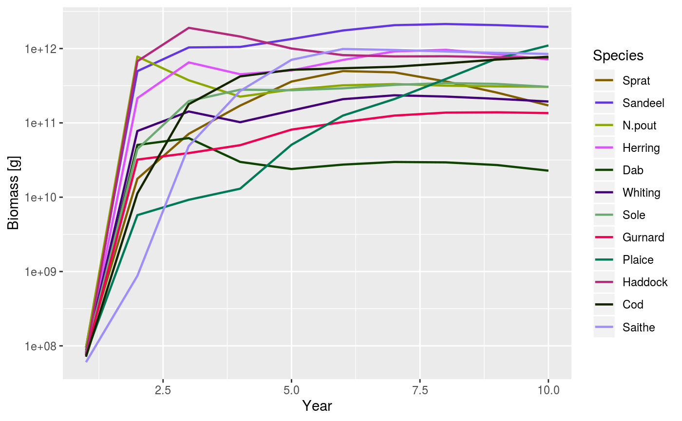

An example of using the plotBiomass() function.

As mentioned above, some of the plot functions plot values against size at a point in time (or averaged over a time period). For these plots it is possible to specify the time step to plot, or the time period to average the values over. The default is to use the final time step. Here we plot the abundance spectra (biomass), averaged over time = 5 to 10:

plotSpectra(sim, time_range = 5:10, biomass=TRUE)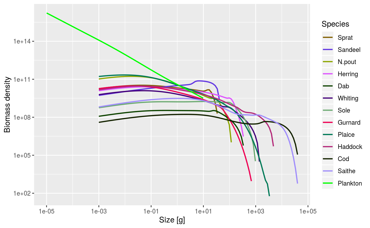

An example of using the plotSpectra() function, plotting values averaged over the period t = 5 to 10.

As mentioned above, and as we have seen several times in this vignette, the generic plot() method has also been overloaded. This produces 5 plots in the same window (plotFeedingLevel(), plotBiomass(), plotPredMort(), plotFMort() and plotSpectra()). It is possible to pass in the same arguments that these individual plots use, e.g. arguments to change the time period over which the data is averaged.

plot(sim)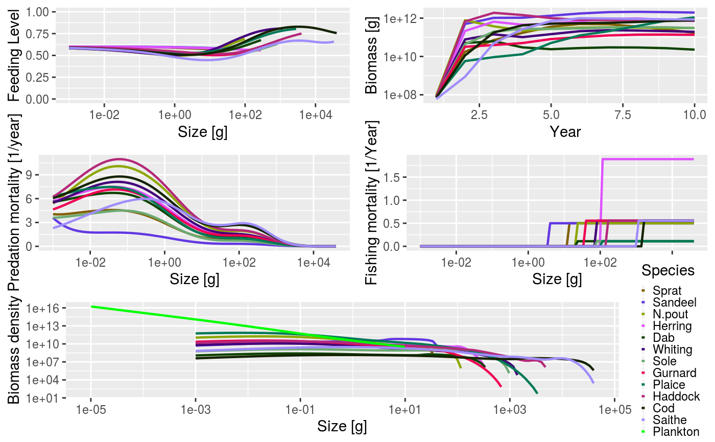

Example output from using the summary plot() method.

The next section describes how to use what we have used to model the North Sea.