A Multi-Species Model Of The North Sea
Edit this page. Source:vignettes/a_multispecies_model_of_the_north_sea.Rmd
a_multispecies_model_of_the_north_sea.RmdIn this section we try to pull everything together with an extended example of a multispecies model for the North Sea. First we will set up the model, project it through time using historical levels of fishing effort, and then examine the results. We then run two different future projection scenarios.
Setting up the North Sea model
The first job is to set up the MizerParams object for the North Sea model. In the previous multispecies examples we have already been using the life-history parameters and the interaction matrix for the North Sea model. We will use them again here but will make some changes. In particular we set up the fishing gears differently.
The parameters and the interaction matrix are stored as *.csv files that need to be read in. We can use the system.file() function to tell us the location of the files. Remember that we need to convert the interaction file into a matrix, hence the use of the as() function.
params_location <- system.file("doc/NS_species_params.csv", package = "mizer")
params_data <- read.csv(params_location)
inter_location <- system.file("doc/inter.csv", package = "mizer")
inter <- as(read.csv(inter_location, row.names = 1), "matrix")
The species in the model are: Sprat, Sandeel, N.pout, Herring, Dab, Whiting, Sole, Gurnard, Plaice, Haddock, Cod, Saithe, which account for about 90% of the total biomass of all species sampled by research trawl surveys in the North Sea. The params_data object is a data.frame with columns for species, w_inf, w_mat, beta, sigma, R_max and k_vb.
We have seen before that only having these columns in the species data.frame is sufficient to make a MizerParams object. Any missing columns will be added and filled with default values by the MizerParams constructor. For example, the data.frame does not include columns for h or gamma. This means that they will be estimated using the k_vb column (see the section on species parameters).
We will use the default stock-recruitment relationship, which is the Beverton-Holt shape. This requires a column R_max in the species data.frame which contains the maximum recruitment flux for each species. This column is already in the params_data data.frame. The values were found through a calibration process which is not covered here but will be added to a later version of this manual.
At the moment, the species data.frame does not contain any information on the selectivity of the gears for the species. By default, the selectivity function is a knife-edge which only takes a single argument, knife_edge_size. In this model we want the selectivity pattern to be a sigmoid shape which more accurately reflects the selectivity pattern of trawlers in the North Sea. The sigmoid selectivity function is expressed in terms of length rather than weight and uses the parameters l25 and l50, which are the lengths at which 25% and 50% of the stock is selected. The length based sigmoid selectivity looks like:
\[\begin{equation} % {#eq:trawl_sel} S_l = \frac{1}{1 + \exp(S1 - S2\ l)} \end{equation}\]
where \(l\) is the length of an individual, \(S_l\) is the selectivity at length, \(S2 = \log(3) / (l50 - l25)\) and \(S1 = l50 \cdot S2\).
This selectivity function is included in mizer as sigmoid_length(). You can see the help page for more details. As well as the arguments l25 and l50, this function has the arguments a and b to convert between length and weight: \(w = a l^b\). This is because the sigmoid selectivity function is defined in terms of length, and the size spectrum model works in terms of weight. As explained in the section on fishing gears and selectivity, all arguments of the selectivity function need to be in the species parameter data.frame. Therefore, columns for l25, l50, a and b need to be added to params_data. We also add a column specifying the name of the selectivity function we wish to use. Note it would probably be easier to add this data directly to the *.csv file and then read it in rather than type it in by hand like we do here:
params_data$sel_func <- "sigmoid_length"
params_data[["l25"]] <- c(7.6, 9.8, 8.7, 10.1, 11.5, 19.8, 16.4, 19.8, 11.5,
    19.1, 13.2, 35.3)
params_data[["l50"]] <- c(8.1, 11.8, 12.2, 20.8, 17.0, 29.0, 25.8, 29.0, 17.0,
    24.3, 22.9, 43.6)
params_data[["a"]] <- c(0.007, 0.001, 0.009, 0.002, 0.010, 0.006, 0.008, 0.004,
0.007, 0.005, 0.005, 0.007)
params_data[["b"]] <- c(3.014, 3.320, 2.941, 3.429, 2.986, 3.080, 3.019, 3.198,
    3.101, 3.160, 3.173, 3.075)
params_data$gear <- params_data$species
Note that we have set up a gear column so that each species will be caught by a separate gear named after the species.
In this model we are interested in projecting forward using historical fishing mortalities. The historical fishing mortality from 1967 to 2010 for each species is stored in the csv file NS_f_history.csv included in the package. As before, we can use read.csv() to read in the data. This reads the data in as a data.frame. We want this to be a matrix so we use the as() function:
f_location <- system.file("doc/NS_f_history.csv", package = "mizer")
f_history <- as(read.csv(f_location, row.names = 1), "matrix")
We can take a look at the first years of the data:
head(f_history)## Sprat Sandeel N.pout Herring Dab Whiting Sole Gurnard
## 1967 0 0 0 1.0360279 0.09417655 0.8294528 0.6502019 0
## 1968 0 0 0 1.7344576 0.07376065 0.8008995 0.7831250 0
## 1969 0 0 0 1.4345001 0.07573638 1.3168280 0.8744095 0
## 1970 0 0 0 1.4342405 0.10537236 1.3473505 0.6389915 0
## 1971 0 0 0 1.8234973 0.08385884 0.9741884 0.8167561 0
## 1972 0 0 0 0.9033768 0.09044461 1.3148588 0.7382834 0
## Plaice Haddock Cod Saithe
## 1967 0.4708827 0.7428694 0.6677456 0.4725102
## 1968 0.3688033 0.7084553 0.6994389 0.4270201
## 1969 0.3786819 1.3302821 0.6917888 0.3844648
## 1970 0.5268618 1.3670695 0.7070891 0.5987086
## 1971 0.4192942 0.9173131 0.7737543 0.4827822
## 1972 0.4522231 1.3279087 0.8393267 0.5796321Fishing mortality is calculated as the product of selectivity, catchability and fishing effort. The values in f_history are absolute levels of fishing mortality. We have seen that the fishing mortality in the mizer simulations is driven by the fishing effort argument passed to the project() function. Therefore if we want to project forward with historical fishing levels, we need to provide project() with effort values that will result in these historical fishing mortality levels.
One of the model parameters that we have not really considered so far is catchability. Catchability is a scalar parameter used to modify the fishing mortality at size given the selectivity at size and effort of the fishing gear. By default catchability has a value of 1, meaning that an effort of 1 results in a fishing mortality of 1 for a fully selected species. When considering the historical fishing mortality, one option is therefore to leave catchability at 1 for each species and then use the f_history matrix as the fishing effort. However, an alternative method is to use the effort relative to a chosen reference year. This can make the effort levels used in the model more meaningful. Here we use the year 1990 as the reference year. If we set the catchability of each species to be the same as the fishing mortality in 1990 then an effort of 1 in 1990 will result in the fishing mortality being what it was in 1990. The effort in the other years will be relative to the effort in 1990.
The catchability can be set by including a catchability column in the species parameters data.frame. Doing this overwrites the default values when the MizerParams constructor is called.
params_data$catchability <- as.numeric(f_history["1990",])Considering the other model parameters, we will use default values for all of the other parameters apart from kappa, the carrying capacity of the plankton spectrum (see see the section on allometric rates). This was estimated along with the values R_max as part of the calibration process.
We now have all the information we need to create the MizerParams object using the species parameters data.frame.
params <- newMultispeciesParams(params_data, inter, kappa = 9.27e10)## Assimilation efficiency `alpha` is not provided in species parameters, so it is set to 0.6.## Starvation mortality coefficient `starv_coef` is not provided in species parameters, so it is set to 10.## Note: No h provided for some species, so using f0 and k_vb to calculate it.## Note: Because you have n != p, the default value is not very good.## Note: No ks column so calculating from critical feeding level.## Note: Using z0 = z0pre * w_inf ^ z0exp for missing z0 values.## Note: Using f0, h, lambda, kappa and the predation kernel to calculate gamma.Setting up and running the simulation
As we set our catchability to be the level of fishing mortality in 1990, before we can run the projection we need to rescale the effort matrix to get a matrix of efforts relative to 1990. To do this we want to rescale the f_history object to 1990 so that the relative fishing effort in 1990 = 1. This is done using R function sweep(). We then check a few rows of the effort matrix to check this has happened:
relative_effort <- sweep(f_history,2,f_history["1990",],"/")
relative_effort[as.character(1988:1992),]
## Sprat Sandeel N.pout Herring Dab Whiting Sole
## 1988 0.8953804 1.2633229 0.8953804 1.214900 1.176678 0.9972560 1.2786517
## 1989 1.1046196 1.2931034 1.1046196 1.232790 1.074205 0.8797926 0.9910112
## 1990 1.0000000 1.0000000 1.0000000 1.000000 1.000000 1.0000000 1.0000000
## 1991 1.1902174 0.8814002 1.1902174 1.108016 1.143110 0.8096927 1.0044944
## 1992 1.2500000 0.8500522 1.2500000 1.316576 1.113074 0.7718676 0.9505618
## Gurnard Plaice Haddock Cod Saithe
## 1988 0.0000000 1.176678 0.9946140 1.045964 1.0330579
## 1989 0.0000000 1.074205 0.8545781 1.060538 1.1223140
## 1990 1.0000000 1.000000 1.0000000 1.000000 1.0000000
## 1991 0.8096927 1.143110 0.7971275 1.001121 0.9619835
## 1992 0.7718676 1.113074 0.8797127 0.970852 1.0528926We could just project forward with these relative efforts. However, the population dynamics in the early years will be strongly determined by the initial population abundances (known as the transient behaviour - essentially the initial behaviour before the long term dynamics are reached). As this is ecology, we don’t know what the initial abundance are. One way around this is to project forward at a constant fishing mortality equal to the mortality in the first historical year until equilibrium is reached. We then can carry on projecting forward using the remaining years of effort. This approach reduces the impact of transient dynamics.
Here we make an initial effort matrix of 100 years at the first effort level. We need to include dimension names for the time dimension. We then stick it on top of the original matrix of historical relative effort using rbind().
initial_effort <- matrix(relative_effort[1,],byrow=TRUE, nrow=100,
    ncol=ncol(relative_effort), dimnames = list(1867:1966))
relative_effort <- rbind(initial_effort,relative_effort)
We now have our parameter object and out matrix of efforts relative to 1990. This includes an initial 100 years of constant relative effort at the 1957 level, followed by the relative effort from 1957 to 2010. We use this effort matrix as the effort argument to the project() function. We use dt = 0.25 (the simulation will run faster than with the default value of 0.1, but tests show that the results are still stable) and save the results every year.
sim <- project(params, effort=relative_effort, dt = 0.25, t_save = 1)Plotting the results, we can see how the biomasses of the stocks change over time. You can see the 100 year period of transients with constant fishing fishing mortality before the historical relative mortality is used from 1967.
plotBiomass(sim)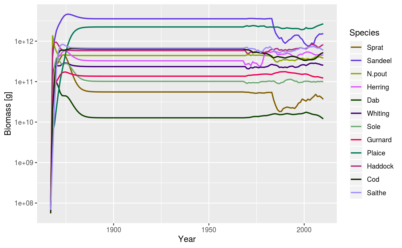
Simulated biomasses of stocks in the North Sea with 100 years of transients.
To explore the state of the community it is useful to calculate indicators of the unexploited community. Therefore we also project forward for 100 years with 0 fishing effort.
sim0 <- project(params, effort=0, dt = 0.5, t_save = 1, t_max = 100)Exploring the model outputs
Here we look at some of the ways the results of the simulation can be explored. We calculate the community indicators mean maximum weight, mean individual weight, community slope and the ‘’large fish indicator’’ (LFI) over the simulation period, and compare them to the unexploited values. We also compare the simulated values of the LFI to a community target based on achieving a high proportion of the unexploited value of the LFI of \(0.8 LFI_{F=0}\).
The indicators are calculated using the functions described in the section about summary functions for MizerSim objects. Here we calculate the LFI and the other community indicators for the unexploited community. When calculating these indicators we only include demersal species and individuals in the size range 10 g to 100 kg, and the LFI is based on species larger than 40 cm. Each of these functions returns a time series. We are interested only in the equilibrium unexploited values so we just select the final time step (year = 100).
demersal_species <- c("Dab","Whiting","Sole","Gurnard","Plaice","Haddock",
    "Cod","Saithe")
lfi0 <- getProportionOfLargeFish(sim0, species = demersal_species,
    min_w = 10, max_w = 100e3, threshold_l = 40)["100"]
mw0 <- getMeanWeight(sim0, species = demersal_species,
    min_w = 10,max_w = 100e3)["100"]
mmw0 <- getMeanMaxWeight(sim0, species = demersal_species,
    min_w = 10, max_w = 100e3)["100","mmw_biomass"]
slope0 <- getCommunitySlope(sim0, species = demersal_species,
    min_w = 10, max_w = 100e3)["100","slope"]
We also calculate the time series of these indicators for the exploited community (we are only interested in the fishing history years, 1967 to 2010, ignoring the transients):
years <- 1967:2010
lfi <- getProportionOfLargeFish(sim, species = demersal_species,
    min_w = 10, max_w = 100e3, threshold_l = 40)[as.character(years)]
mw <- getMeanWeight(sim, species = demersal_species,
    min_w = 10, max_w = 100e3)[as.character(years)]
mmw <- getMeanMaxWeight(sim, species = demersal_species,
    min_w = 10, max_w = 100e3)[as.character(years),"mmw_biomass"]
slope <- getCommunitySlope(sim, species = demersal_species,
    min_w = 10, max_w = 100e3)[as.character(years),"slope"]
We can plot the exploited and unexploited indicators, along LFI reference level. Here we do it using ggplot2 which uses data.frames. We make three data.frames (one for the time series, one for the unexploited levels and one for the reference level): Each data.frame is a data.frame of each of the measures, stacked on top of each other.
library(ggplot2)
# Simulated data
community_plot_data <- rbind(
    data.frame(year = years, measure = "LFI", data = lfi),
    data.frame(year = years, measure = "Mean Weight", data = mw),
    data.frame(year = years, measure = "Mean Max Weight", data = mmw),
    data.frame(year = years, measure = "Slope", data = slope))
# Unexploited data
community_unfished_data <- rbind(
    data.frame(year = years, measure = "LFI", data = lfi0[[1]]),
    data.frame(year = years, measure = "Mean Weight", data = mw0[[1]]),
    data.frame(year = years, measure = "Mean Max Weight", data = mmw0[[1]]),
    data.frame(year = years, measure = "Slope", data = slope0[[1]]))
# Reference level
community_reference_level <-
    data.frame(year=years, measure = "LFI", data = lfi0[[1]] * 0.8)
# Build up the plot
p <- ggplot(community_plot_data) + geom_line(aes(x=year, y = data)) +
    facet_wrap(~measure, scales="free")
p <- p + geom_line(aes(x=year,y=data), linetype="dashed",
    data = community_unfished_data)
p + geom_line(aes(x=year,y=data), linetype="dotted",
    data = community_reference_level)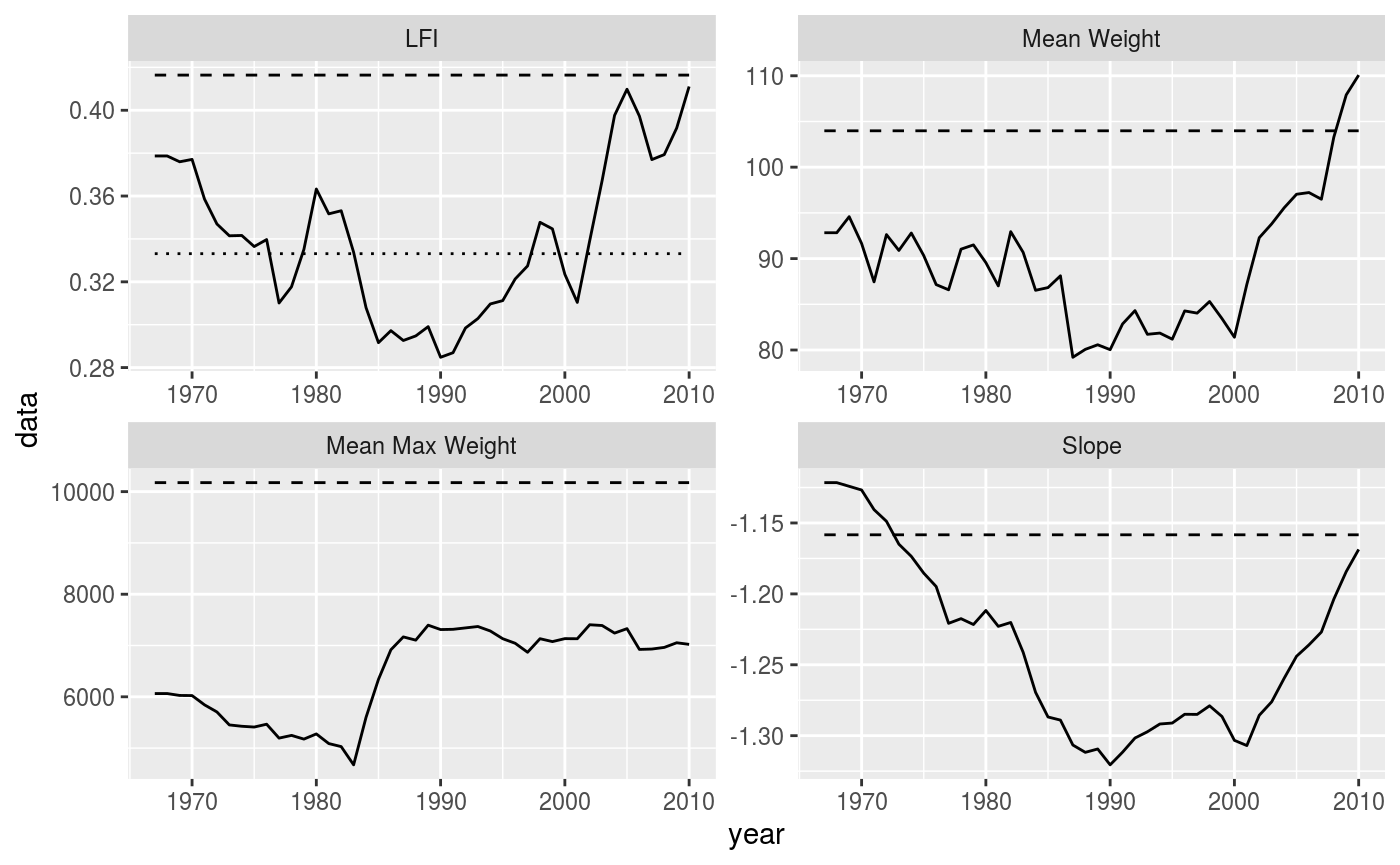
Historical (solid) and unexploited (dashed) and reference (dotted) community indicators for the North Sea multispecies model.
According to our simulations, historically the LFI in the North Sea has been below the reference level.
Future projections
As well as investigating the historical simulations, we can run projections into the future. Here we run two projections to 2050 with different fishing scenarios.
- Continue fishing at 2010 levels (the status quo scenario).
- From 2010 to 2015 linearly change the fishing mortality to approach \(F_{MSY}\) and then continue at \(F_{MSY}\) until 2050.
Rather than looking at community indicators here, we will calculate the SSB of each species in the model and compare the projected levels to a biodiversity target based on the reference point \(0.1 SSB_{F=0}.\)
Before we can run the simulations, we need to set up arrays of future effort. We will continue to use effort relative to the level in 1990. Here we build on our existing array of relative effort to make an array for the first scenario. Note the use of the t() command to transpose the array. This is needed because R recycles by rows, so we need to build the array with the dimensions rotated to start with. We make an array of the future effort, and then bind it underneath the relative_effort array used in the previous section.
scenario1 <- t(array(relative_effort["2010",], dim=c(12,40),
    dimnames=list(NULL,year = 2011:2050)))
scenario1 <- rbind(relative_effort, scenario1)
The relative effort array for the second scenario is more complicated to make and requires a little bit of R gymnastics (it might be easier for you to prepare this in a spreadsheet and read it in). For this one we need values of \(F_{MSY}\).
fmsy <- c(Sprat = 0.2, Sandeel = 0.2, N.pout = 0.2, Herring = 0.25, Dab = 0.2,
    Whiting = 0.2, Sole = 0.22, Gurnard = 0.2, Plaice = 0.25, Haddock = 0.3,
    Cod = 0.19, Saithe = 0.3)
scenario2 <- t(array(fmsy, dim=c(12,40), dimnames=list(NULL,year = 2011:2050)))
scenario2 <- rbind(relative_effort, scenario2)
for (sp in dimnames(scenario2)[[2]]){
    scenario2[as.character(2011:2015),sp] <- scenario2["2010",sp] +
        (((scenario2["2015",sp] - scenario2["2010",sp]) / 5) * 1:5)
}
Both of our new effort scenarios still include 100 years at the 1967 level to reduce the impact of the transient behaviour. We are now ready to project the two scenarios.
sim1 <- project(params, effort = scenario1, dt = 0.25, t_save = 1)
sim2 <- project(params, effort = scenario2, dt = 0.25, t_save = 1)
We can now compare the projected SSB values in both scenarios to the biodiversity reference points. First we calculate the biodiversity reference points (from the final time step in the unexploited sim0 simulation):
ssb0 <- getSSB(sim0)["100",]Now we build a data.frame of the projected SSB for each species, ignoring the transients. We make use of the melt() function in the very useful reshape2 package (REF).
library(reshape2)
years <- 1967:2050
ssb1 <- getSSB(sim1)[as.character(years),]
ssb2 <- getSSB(sim2)[as.character(years),]
ssb1_df <- melt(ssb1)
ssb2_df <- melt(ssb2)
ssb_df <- rbind(
    cbind(ssb1_df, scenario = "Scenario 1"),
    cbind(ssb2_df, scenario = "Scenario 2"))
ssb_unexploited_df <- cbind(expand.grid(
    sp = names(ssb0),
    time = 1967:2050),
    value = as.numeric(ssb0),
    scenario = "Unexploited")
ssb_reference_df <- cbind(expand.grid(
    sp = names(ssb0),
    time = 1967:2050),
    value = as.numeric(ssb0*0.1),
    scenario = "Reference")
ssb_all_df <- rbind(
    ssb_df,
    ssb_unexploited_df,
    ssb_reference_df)
p <- ggplot(ssb_all_df) +
    geom_line(aes(x = time, y = value, colour = scenario)) +
    facet_wrap(~sp, scales = "free", nrow = 4)
p + theme(legend.position = "none")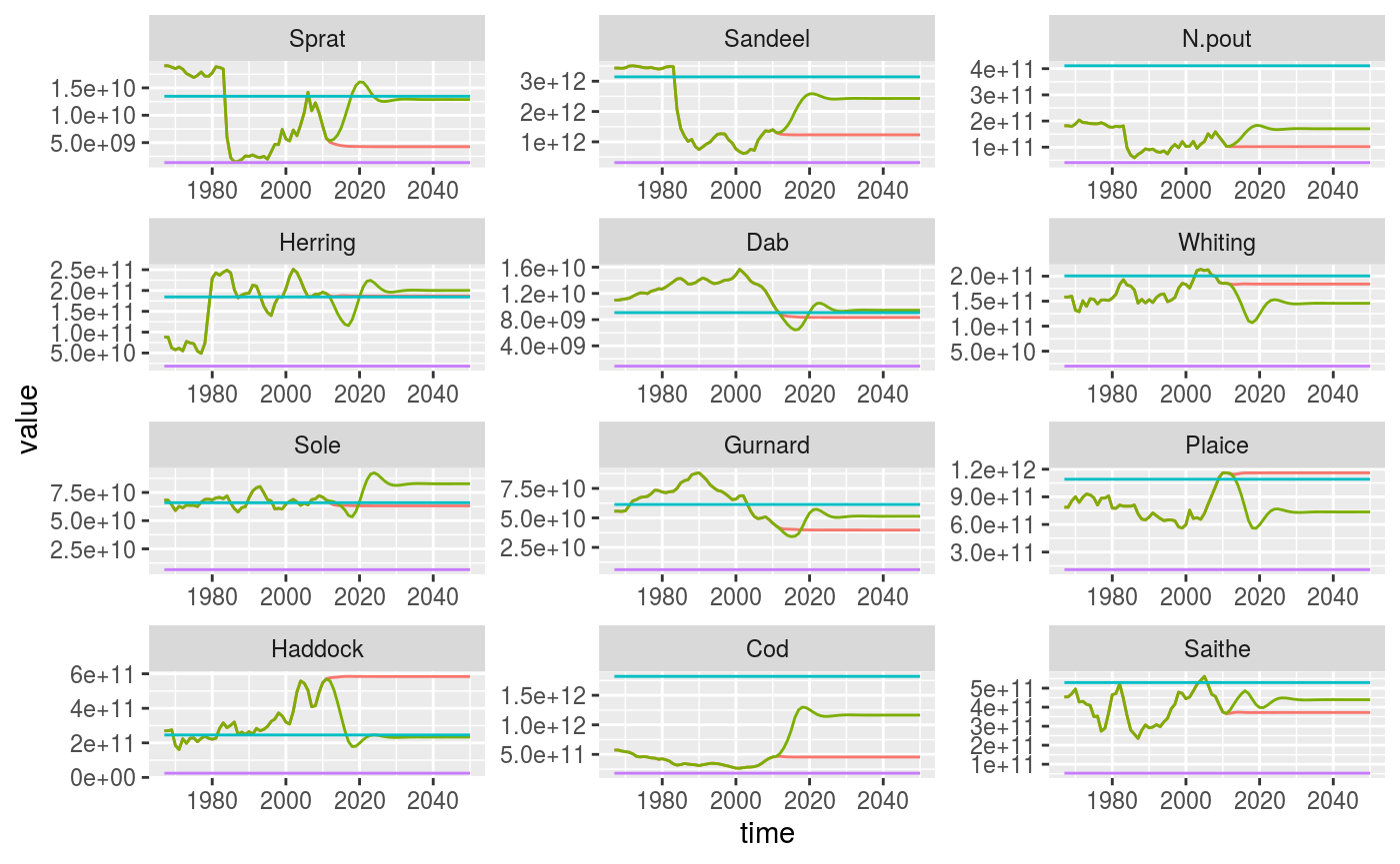
Historical and projected SSB under two fishing scenarios. Status quo (red), Fmsy (yellow). Unexploited (blue) and reference levels (purple) are also shown.