8 Ordinary Differential Equations

The mathematical discipline of differential equations furnishes the explanation of all those elementary manifestations of nature which involve time.
–Norwegian Mathematician Sophus Lie

The topic of this chapter is to find approximate solutions to ordinary differential equations.

Let us briefly recall what an ordinary differential equation (ODE) is. A rather arbitrarily chosen example for an ODE (here, of second order) is \[ y''(x) + 4 y'(x) + \sqrt[3]{y(x)} + \cos(x) = 0. \tag{8.1}\] Equations like this are normally satisfied by many functions $y(x)$: the problem has many solutions. In order to specify a uniquely solvable problem, one needs to fix initial values, i.e., the value of $y$ and its first derivative at some point, say, at $x=0$: \[ y''(x) + 4 y'(x) + \sqrt[3]{y(x)} + \cos(x) = 0, \quad y(0)=1,\; y'(0)=-2. \tag{8.2}\] This is a so-called initial-value problem (IVP). Another variant is to specify the value of $y(x)$, but not of its derivative, at two different points: \[ y''(x) + 4 y'(x) + \sqrt[3]{y(x)} + \cos(x) = 0, \quad y(0)=2,\; y(1)=1. \tag{8.3}\] This is called a boundary value problem (BVP).

Both IVPs and BVPs have a unique solution (under certain mathematical conditions). However, while one can show on abstract grounds that these solutions exist, it is often not practicable to find an explicit expression for them. The best one can hope for is to approximate the solution numerically.

So what is a numerical solution to a differential equation?
When solving a differential equation with analytic techniques the goal is to find an expression for the solution in terms of known functions. In a numerical solution the goal is typically to divide the domain for the solution function into a fine partition by introducing a grid of points, just like we did with numerical differentiation and integration, and then to approximate the solution to the differential equation at each point in that partition. Hence, the end result will be a list of approximate solution values at the grid points.

In this chapter we will examine some of the more common ways to create approximations of solutions to initial value problems. Moreover, we will lean heavily on Taylor Series to give us ways to accurately measure the order of the errors that we make in the process.

In this chapter we will often think of the argument of the function described by the ODE as time, but of course the methods are agnostic to the interpretation of the independent variable.

8.1 Euler’s Method

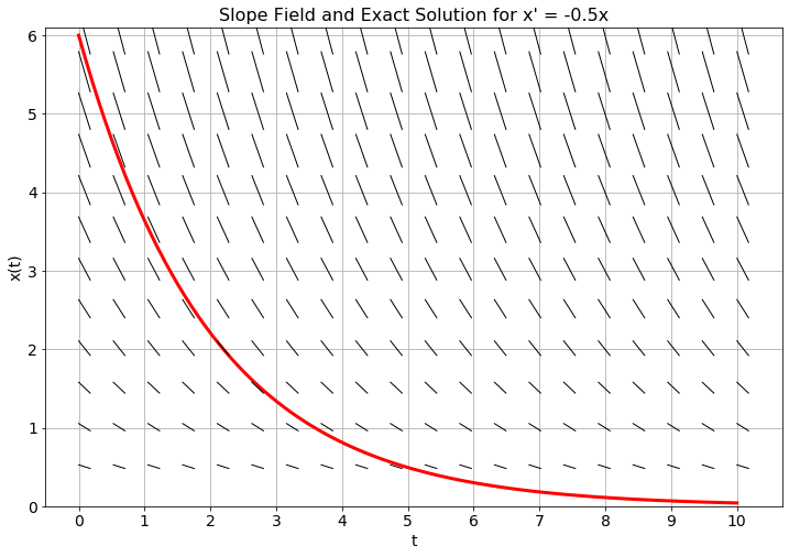
Exercise 8.1 Consider the differential equation $x' = -0.5x$ with the initial condition $x(0) = 6$.

Since we know that $x(0) = 6$ and we know that $x'(0) = -0.5 x(0)$ we can approximate the value of $x$ at some future time step. Let us go 1 unit forward in time. That is, approximate $x(1)$ knowing that $x(0) = 6$ and $x'(0) = -3$.
Hint: We know a value, a slope, and the size of the step that we would like to move in the $t$ direction. \[\begin{equation} x(1) \approx \underline{\hspace{1in}} \end{equation}\]
Use your answer from part (a) for time $t=1$ to approximate the $x$ value at time $t=2$. Then use that value to approximate the value at time $t=3$. Repeat the process to approximate the value of $x$ at times $t=2, 3, 4$. Record your answers in the table below. Then find the analytic solution to this differential equation and record the $x$ values at the appropriate times.

$t$	0	1	2	3	4
Approximation of $x(t)$	6
Exact value of $x(t)$	6

The “approximations of $x$” that you found in part (b) are a numerical approximation of the solution to the differential equation. You should notice that your numerical solution is pretty far off from the actual solution for most values of $t$. Why? What could be the sources of this error and how could we fix it? Once you have an idea of how to fix it, put your idea into action and devise some measurement of error to analyse your results.
In Figure 8.1 you will see a slope field and the exact solution to the differential equation $x' = -0.5x$ with $x(0) = 6$. Mark your approximate solutions at times $t=1$, $t=2$, $\ldots$, $t=4$ on the plot and connect them with straight lines.
1. Why are we using straight lines to connect the points?
2. What do you notice about your approximate solutions?
3. Why is it helpful to have the slope field in the background on this plot?

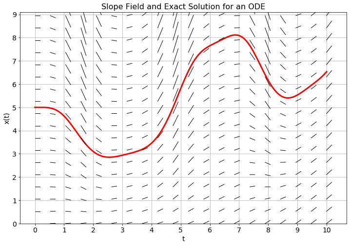
Figure 8.1: Plot your approximate solution on top of the slope field and the exact solution.

Exercise 8.2 In Figure 8.2 you see the analytic solution with initial condition $x(0)=5$ and a slope field for an unknown differential equation.

Use the slope field and a step size of $\Delta t=1$ to plot approximate solution values at $t=1$, $t=2$, $\ldots$, $t=10$. Connect your points with straight lines. The collection of line segments that you just drew is an approximation to the solution of the unknown differential equation.
Use the slope field and a step size of $\Delta t = 0.5$ to plot approximate solution values at $t=0.5$, $t=1$, $t=1.5$, $\ldots$, $t=10$. Again, connect your points with straight lines to get an approximation of the solution to the unknown differential equation.
If you could take $\Delta t$ to be very very small, what difference would you see graphically between the exact solution and your collection of line segments? Why?

Figure 8.2: Plot your approximate solution on top of the slope field and the exact solution.

The notion of approximating solutions to differential equations is simple in principle:

make a discrete approximation to the derivative and
step forward through time as a difference equation.

The challenging part is making the approximation to the derivative(s). There are many methods for approximating derivatives, and that is exactly where we will start.

Definition 8.1 (Euler’s Method) Euler’s Method is a technique for approximating the solution to the differential equation $x'(t) = f(t,x(t))$. Recall from Exercise 5.6 that the first derivative of a function can be discretized as \[\begin{equation} x'(t) = \frac{x(t+h) - x(t)}{h} + \mathcal{O}(h) \end{equation}\] where $h = \Delta t$ is the step size (or the size of each partition in the domain), so the differential equation $x'(t) = f(t,x(t))$ becomes \[\begin{equation} \frac{x(t+h) - x(t)}{h} \approx f(t,x(t)). \end{equation}\] Rewriting as a difference equation, letting $x_{n+1} = x(t_n+h)$ and $x_n = x(t_n)$, we get \[\begin{equation} x_{n+1} = x_n + h f(t_n,x_n) \end{equation}\]

A way to think about Euler’s method is that at a given point, the slope is approximated by the value of the right-hand side of the differential equation and then we step forward $h$ units in time following that slope. Figure 8.3 shows a depiction of the idea. Notice in the figure that in regions of high curvature Euler’s method will deviate a lot from the exact solution to the differential equation. However, taking the limit as $h$ tends to $0$ theoretically gives the exact solution at the trade off of needing infinite computational resources.

Figure 8.3: Numerical solutions to a differential equation using Euler’s method.

Exercise 8.3 Why would Euler’s method do poorly in regions where the solution exhibits high curvature?

Exercise 8.4 🎓 Consider the differential equation $x'(t) = -2x(t)/3 + 4t$ with initial condition $x(0)=6$. By hand perform four steps of the Euler method with stepsize $h=1/2$ to obtain an approximation for $x(1/2),x(1),x(3/2)$ and $x(2)$.

Exercise 8.5 🎓 Write code to implement Euler’s method for initial value problems. Your function should accept as input a Python function $f(t,x)$, an initial condition, a start time, an end time, and the value of $h = \Delta t$. The output should be vectors for $t$ and $x$ that you can easily plot to show the numerical solution. The code below will get you started.

def euler1d(f, x0, t0, tmax, dt):
    """
    Solves a first-order ordinary differential equation using the Euler method.

    Parameters:
        f    : function, the function defining the differential equation. It should 
               take two arguments, the independent variable t and the dependent 
               variable x, and return the derivative of x with respect to t.
        x0   : float, the initial value of the dependent variable.
        t0   : float, the initial value of the independent variable.
        tmax : float, the maximum value of the independent variable.
        dt   : float, the time step.

    Returns:
       tuple containing two numpy arrays:
            - t : vector of time values.
            - x : vector of solution values at each time value.
    """
    # set up the grid with points from t0 to tmax with stepsize dt
    t = np.aranbe(???, ???, ???)
    # set up an array for x that is the same size as t
    x = np.zeros(len(t))
    # fill in the initial condition
    x[0] = ???
    for n in range(???): # think about how far we should loop
        # advance the solution forward in time with Euler
        x[n+1] = ???
    return t, x

Exercise 8.6 Test your code from the previous exercise on a first order differential equation where you know an analytic solution. For example you could use the differential equation \[\begin{equation} x' = -\frac{1}{3}x+\sin(t) \quad \text{where} \quad x(0) = 1. \end{equation}\] This has the analytic solution \[\begin{equation} x(t) = \frac{1}{10} \left( 19 e^{-t/3} + 3\sin(t) - 9\cos(t) \right). \end{equation}\] Make a plot of the approximate solution and the exact solution on the same plot for $t\in[0,10]$ The partial code below should get you started.

import numpy as np
import matplotlib.pyplot as plt

# Define the function giving x' in terms of t and x
f = lambda t, x: ???
x0 = ???   # initial condition
t0 = ???   # initial time
tmax = ??? # final time
dt = ???   # time step (your choice, but make it small)
t, x = euler1d(f, x0, t0, tmax, dt)
plt.plot(t, x, 'b-', label='Euler')

# Define a function giving the analytic solution
x_exact = lambda t: ???
# We will plot the exact solution at a higher resolution
t_hires = np.linspace(t0, tmax, 100)
plt.plot(t_highres, x_exact(t_highres), 'r--', label='Exact')
plt.grid()
plt.show()

Experiment with different values for dt and see how the numerical solution changes.

Exercise 8.7 The goal of this problem will be to compare the maximum error when you solve the differential equation from the previous exercise on the interval $t \in [0,10]$ with the Euler method for various values of $\Delta t$.

Write a function that produces a plot with the value of $\Delta t$ on the horizontal axis and the value of the associated absolute error on the vertical axis. You should use a log-log plot. Obviously you will need to run your code many times at many different values of $\Delta t$ to build your data set. The following incomplete code will get you started.

# Create vector with different step sizes
dt = 10**(-np.linspace(0, 4, 50))
# Create vector with the same size as dt for holding the errors
errors = np.zeros_like(dt)
# Loop over the different step sizes to calculate the errors
for i in range(len(dt)):
    # Approximate the solution with Euler's method
    t, x = euler1d(f, x0, t0, tmax, dt[i])
    errors[i] = ??? # Calculate maximum absolute error

# Plot the errors with logarithmic axes
plt.loglog(dt, errors)
plt.xlabel('Step size')
plt.ylabel('Maximum error')
plt.grid()

What does the plot tell you? In general, if you were to divide your value of $\Delta t$ by 10, how much approximately does that reduce the error?

Exercise 8.8 Shelby solved a first order ODE $x' = f(t,x)$ using Euler’s method with a step size of $dt = 0.1$ on a domain $t \in [0,3]$. To test her code she used a differential equation where she new the exact analytic solution and she found the maximum absolute error on the interval to be $0.15$. Jackson then solves the exact same differential equation, on the same interval, with the same initial condition using Euler’s method and a step size of $dt = 0.01$. What would be your best estimate of Jackson’s maximum absolute error?

Theorem 8.1 Euler’s method is a first order method for approximating the solution to the differential equation $x' = f(t,x)$. Hence, if the step size $h$ of the partition of the domain were to be divided by some positive constant $M$ then the maximum absolute error between the numerical solution and the exact solution would ???
(Complete the last sentence.)

8.2 Higher-order equations and systems of equations

Exercise 8.9 (Harmonic oscillator) If a mass is hanging from a spring then Newton’s second law, $\sum F=ma$, gives us the differential equation $mx'' = F_{restoring} + F_{damping}$ where $x$ is the displacement of the mass from equilibrium, $m$ is the mass of the object hanging from the spring, $F_{restoring}$ is the force pulling the mass back to equilibrium, and $F_{damping}$ is the force due to friction or air resistance that slows the mass down.

Which of the following is a good candidate for a restoring force in a spring? Defend your answer.
1. $F_{restoring} = kx$: The restoring force is proportional to the displacement away from equilibrium.
2. $F_{restoring} = kx'$: The restoring force is proportional to the velocity of the mass.
3. $F_{restoring} = kx''$: The restoring force is proportional to the acceleration of the mass.
Which of the following is a good candidate for a damping force in a spring? Defend your answer.
1. $F_{damping} = bx$: The damping force is proportional to the displacement away from equilibrium.
2. $F_{damping} = bx'$: The damping force is proportional to the velocity of the mass.
3. $F_{damping} = bx''$: The damping force is proportional to the acceleration of the mass.
Put your answers to parts (1) and (2) together and simplify to form a second-order differential equation for position: \[\begin{equation} \underline{\hspace{0.25in}} x'' = \underline{\hspace{0.25in}} x' + \underline{\hspace{0.25in}} x \end{equation}\]
🎓 If we want to solve a second order differential equation numerically we need to convert it to first order differential equations (Euler’s method is only designed to deal with first order differential equations, not second order). To do so we can introduce a new variable, $x_1$, such that $x_1 = x'$. For the sake of notational consistency we define $x_0 = x$. The result is a system of first-order differential equations. \[\begin{equation} \begin{aligned} x_0' &= x_1 \\ x_1' &= \underline{\hspace{2in}}\end{aligned} \end{equation}\]
The code and Euler’s method algorithm that we have created thus far in this chapter are only designed to work with a single differential equation instead of a system, so we need to make some modifications. We can discretize the system of differential equations using Euler’s method so that \[\begin{equation} \boldsymbol{x}' = F(t,\boldsymbol{x}) \end{equation}\] where $F$ is a function that accepts a vector of inputs, plus time, and returns a vector of outputs. In the context of this particular problem, \[\begin{equation} F(t,\boldsymbol{x}) = \begin{pmatrix} x_0' \\ x_1' \end{pmatrix} = \begin{pmatrix} x_1 \\ \underline{\hspace{1in}} \end{pmatrix} \end{equation}\]
We now need to discretize the derivatives in the system. As with 1D Euler’s method, we will use a first-order approximation of the first derivative so that \[\begin{equation} \frac{\boldsymbol{x}_{n+1} - \boldsymbol{x}_n }{h} = F(t_n,\boldsymbol{x}_n) + \mathcal{O}(h). \end{equation}\] Rearranging and solving for $\boldsymbol{x}_{n+1}$ gives \[\begin{equation} \boldsymbol{x}_{n+1} = \underline{\hspace{0.5in}} + h F( \underline{\hspace{0.25in}} , \underline{\hspace{0.25in}}). \end{equation}\]
The following Python function will implement Euler’s method. Complete the code.

def euler(F, x0, t0, tmax, dt):
    """
    Solves a system of first-order ordinary differential equations 
    using the Euler method.

    Parameters:
        F : function, the function defining the system of differential equations. 
            It should take two arguments, the independent variable t and the 
            dependent variable x (as a 1D numpy array), and return the 
            derivative of x with respect to t (as a 1D numpy array).
        x0 : numpy vector, the initial values of the dependent variables.
        t0 : float, the initial value of the independent variable.
        tmax : float, the maximum value of the independent variable.
        dt : float, the time step.

    Returns:
        tuple containing two numpy arrays:
            - t : vector of time values.
            - x : array of solutions at each time value. Each column of x 
                  corresponds to a different dependent variable.
    """
    # set up the grid with points from t0 to tmax with stepsize dt
    t = ???
    # set up array x with one row for each dependent variable and one column
    # for each grid point
    x = np.zeros((len(t), len(x0))) 
    # store the initial condition in the first row of x
    x[0, :] = x0 
    # loop over the different time steps
    for n in range(???):
        x[n+1, :] = x[???, ???] + dt * F(t[???], x[???, ???])
    return t, x

To use the euler() function to solve the system of equations from part (4), complete the following code. Use a mass of $m=2$kg, a damping force of $b=40$kg/s, and a spring constant of $k=128$N/m. Consider an initial position of $x=0$ (equilibrium) and an initial velocity of $x_1 = 0.6$m/s.

m = 2
b = 40
k = 128
F = lambda t, x: np.array([x[1], ???])
x0 = [???, ???] # initial conditions
t0 = 0
tmax = 5  # pick something reasonable here
dt = 0.01 # your choice.  pick something small
t, x = euler(F, x0, t0, tmax, dt)

🎓 Complete the following code to make a plot that shows both position and velocity versus time.

plt.plot(t, x[???, ???], 'b-', t, x[???, ???], 'r--')
plt.grid()
plt.title('Time Evolution of Position and Velocity')
plt.legend(['which legend entry here','which legend entry here'])
plt.xlabel('time')
plt.ylabel('position and velocity')
plt.show()

Complete the following code to make a second plot, called a phase plot, that shows position versus velocity. In a phase plot, time is implicit (not one of the axes).

plt.plot(x[???, ???], x[???, ???])
plt.grid()
plt.title('Phase Plot')
plt.xlabel('???')
plt.ylabel('???')
plt.show()

Exercise 8.10 (A Lotka-Volterra Predator-Prey Model) Let $x_0(t)$ denote the number of rabbits (prey) and $x_1(t)$ denote the number of foxes (predator) at time $t$. The relationship between the species can be modelled by the classic 1920’s Lotka-Volterra Model: \[\begin{equation} \left\{ \begin{array}{ll} x_0' &= \alpha x_0 - \beta x_0 x_1 \\ x_1' &= \delta x_0 x_1 - \gamma x_1 \end{array} \right. \end{equation}\] where $\alpha, \beta, \gamma,$ and $\delta$ are positive constants. For this problems take $\alpha =1$, $\beta \approx 0.1$, $\gamma =1$, and $\delta =0.1$.

First rewrite the system of ODEs in the form $\boldsymbol{x}' = F(t,\boldsymbol{x})$ so you can use your euler() code.
Modify your code from the previous problem so that it works for this problem. Use tmax = 20 and dt = 0.05. Start with initial conditions $x_0(0)=10$ rabbits and $x_1(0)=5$ foxes.
Create the time evolution plot. What does this plot tell you in context?
Create a phase plot. What does this plot tell you in context?
If you decrease the step size by a factor of 10, what do you see in the two plots? Why?

Exercise 8.11 (The SIR Model) A classic model for predicting the spread of a virus or a disease is the SIR Model. In these models, $S$ stands for the proportion of the population which is susceptible to the virus, $I$ is the proportion of the population that is currently infected with the virus, and $R$ is the proportion of the population that has recovered from the virus. The idea behind the model is that

Susceptible people become infected by having interaction with the infected people. Hence, the rate of change of the susceptible people is proportional to the number of interactions that can occur between the $S$ and the $I$ populations.

\[\begin{equation} S' = -\beta SI. \end{equation}\]

The infected population gains people from the interactions with the susceptible people, but at the same time, infected people recover at a predictable rate. \[\begin{equation} I' = \beta SI - \gamma I. \end{equation}\]
The people in the recovered class are then immune to the virus, so the recovered class $R$ only gains people from the recoveries from the $I$ class. \[\begin{equation} R' = \gamma I. \end{equation}\]

Find a numerical solution to the system of equations using your euler() function. Use the parameters $\beta = 0.0003$ and $\gamma = 0.1$ with initial conditions $S(0) = 999$, $I(0) = 1$, and $R(0) = 0$. Plot the solution against time. Explain all three curves in context.

8.3 The Midpoint Method

Now we get to improve upon Euler’s method. There is a long history of wonderful improvements to the classic Euler’s method – some that work in special cases, some that resolve areas where the error is going to be high, and some that are great for general purpose numerical solutions to ODEs with relatively high accuracy. In this section we will make a simple modification to Euler’s method that has a surprisingly great pay-off in the error rate.

Exercise 8.12 In Euler’s method, if we are at the point $t_n$ then we approximate the slope $x'(t_n) = f(t_n,x_n)$ and use the slope to propagate forward one time step. As you have seen, this method can lead to an overshooting of the exact solution in regions of high curvature. It would be nice to be able to look into the future and get a better approximation of the slope so that we did not miss upcoming curvature. If you could build such a method that looks in to the future, finds a slope in the future, and then uses that slope (instead of the slope from Euler’s method) to advance forward in time, how far into the future would you look? Why?

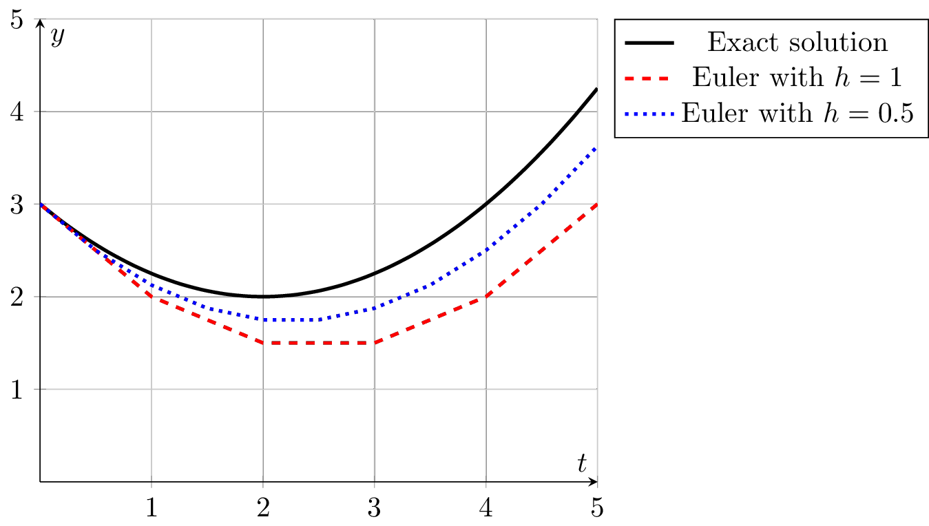
Exercise 8.13 Let us return to the simple differential equation $x' = -0.5x$ with $x(0) = 6$ that we saw in Exercise 8.1. Now we will propose a slightly different method for approximating the solution.

At $t=0$ we know that $x(0)=6$. If we use the slope at time $t=0$ to step forward in time then we will get the Euler approximation of the solution. Consider this alternative approach:
- Use the slope at time $t=0$ and move half a step forward.
- Find the slope at the half-way point
- Then use the slope from the half way point to go a full step forward from time $t=0$.
Perhaps a bit confusing …let us build this idea together:
- What is the slope at time $t=0$? $x'(0) = \underline{\hspace{0.5in}}$
- Use this slope to step a half step forward and find the $x$ value: $x(0.5) \approx \underline{\hspace{0.5in}}$
- Now use the differential equation to find the slope at time $t=0.5$. $x'(0.5) = \underline{\hspace{0.5in}}$
- Now take your answer from the previous step, and go one full step forward from time $t=0$. What $x$ value do you end up with?
- Your answers to the previous bullets should be: $x'(0) = -3$, $x(0.5) \approx 4.5$, $x'(0.5) = -2.25$, so if we take a full step forward with slope $m=-2.25$ starting from $t=0$ we get $x(1) \approx 3.75$.
Repeat the process outlined in part (a) to approximate the solution to the differential equation at times $t=2, 3, 4$. Also record the exact answer at each of these times by noting that the exact solution is $x(t) = 6e^{-0.5t}$.

$t$	0	1	2	3	4
Euler approx of $x(t)$	6
New approx of $x(t)$	6
Exact value of $x(t)$	6

Draw a clear picture of what this method is doing in order to approximate the slope at each individual step.
How does your approximation compare to the Euler approximation that you found in Exercise 8.1?

Definition 8.2 (The Midpoint Method) The midpoint method is defined by first taking a half step with Euler’s method to approximate a solution at time $t_{n+1/2}$ There is no grid point at $t_{n+1/2}$ so we define this as \[ t_{n+1/2} = (t_n + t_{n+1})/2. \] We then take a full step using the value of $f$ at $t_{n+1/2}$ and the approximate $x_{n+1/2}$. \[ \begin{split} x_{n+1/2} &= x_n + \frac{h}{2} f(t_n,x_n) \\ x_{n+1} &= x_n + h f(t_{n+1/2},x_{n+1/2}) \end{split} \]

Exercise 8.14 🎓 As in in Exercise 8.4, consider the differential equation $x'(t) = -2x(t)/3 + 4t$ with initial condition $x(0)=6$. By hand perform one step of the midpoint method with stepsize $h=1$ to obtain an approximation for $x(1)$.

Exercise 8.15 Complete the code below to implement the midpoint method in one dimension.

def midpoint1d(f, x0, t0, tmax, dt):
    """
    Solves a first-order ordinary differential equation using 
    the midpoint method.

    Parameters:
        f    : function, the function defining the differential equation. It should 
               take two arguments, the independent variable t and the dependent 
               variable x, and return the derivative of x with respect to t.
        x0   : float, the initial value of the dependent variable.
        t0   : float, the initial value of the independent variable.
        tmax : float, the maximum value of the independent variable.
        dt   : float, the time step.

    Returns:
       tuple containing two numpy arrays:
            - t : vector of time values.
            - x : vector of solution values at each time value.
    """
    t = ??? # build the times
    x = ??? # build an array for the x values
    x[0] = # save the initial condition
    # On the next line: be careful about how far you're looping
    for n in range(???): 
        slope = ??? # get the slope at the current point
        x_halfstep = ??? # take a half step forward
        x[n+1] = ??? # take a full step forward
    return t, x

Test your code on several differential equations where you know the solution (just to be sure that it is working).

f = lambda t, x: # your ODE right hand side goes here
x0 = # initial condition
t0 = 0
tmax = # ending time (up to you)
dt = # pick something small
t, x = midpoint1d(???, ???, ???, ???, ???)
plt.plot(???, ???, ???)
x_exact = lambda t: # your exact solution goes here
plt.plot(???, ???, ???)
plt.legend(['Midpoint', 'Exact'])
plt.grid()
plt.show()

Exercise 8.16 The goal in building the midpoint method was to hopefully capture some of the upcoming curvature in the solution before we overshot it. Consider the differential equation $x' = -\frac{1}{3}x + \sin(t)$ with initial condition $x(0) = 1$ on the domain $t \in [0,10]$ as in Exercise 8.6. First get a numerical solution with Euler’s method using $\Delta t = 1$. Then get a numerical solution with the midpoint method using the same value for $\Delta t = 1$. Plot the two solutions on top of each other along with the exact solution \[\begin{equation} x(t) = \frac{1}{10} \left( 19e^{-t/3} + 3\sin(t) - 9\cos(t) \right). \end{equation}\] What do you observe?

Exercise 8.17 🎓 Repeat Exercise 8.7 with the midpoint method. Compare your results to what you found with Euler’s method.

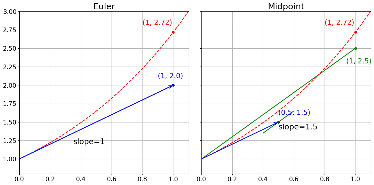
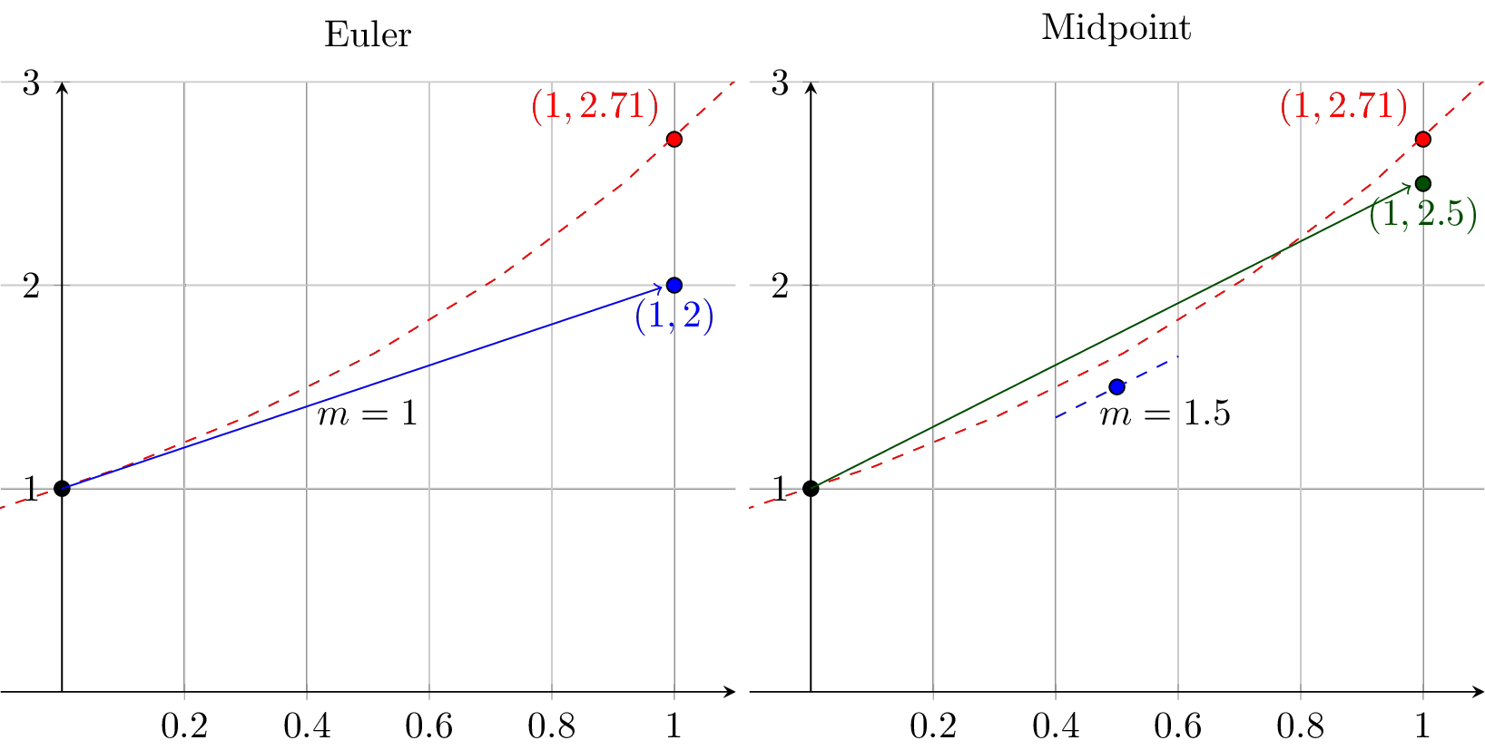
Exercise 8.18 We have studied two methods thus far: Euler’s method and the Midpoint method. In Figure 8.5 we see a graphical depiction of how each method works on the differential equation $y' = y$ with $\Delta t = 1$ and $y(0) = 1$. The exact solution at $t=1$ is $y(1) = e^1 \approx 2.718$ and is shown in red in each figure. The methods can be summarized in the table below.

Discuss what you observe as the pros and cons of each method based on the table and on the Figure.

Euler’s Method	Midpoint Method
1. Get the slope at time $t_n$	1. Get the slope at time $t_n$
2. Follow the slope for time $\Delta t$	2. Follow the slope for time $\Delta t/2$
	3. Get the slope at the point $t_n + \Delta t/2$
	4. Follow the new slope from time $t_n$ for time $\Delta t$

When might you want to use Euler’s method instead of the midpoint method? When might you want to use the midpoint method instead of Euler’s method?

Figure 8.4: Graphical depictions of two numerical methods. Euler (left) and Midpoint (right). The exact solution is shown in red.

Figure 8.5: Graphical depictions of two numerical methods: Euler (left) and Midpoint (right). The exact solution is shown in red.

Exercise 8.19 (Midpoint Method in Several Dimensions) 🎓 Write a function midpoint() that can solve a system of first-order ordinary differential equations using the midpoint method. Base your code on the euler() code from Exercise 8.9 . You should only have to add one line of code and then be careful about the size of the arrays that are in play. Test your code on several problems. Compare and contrast what you see with your Euler solutions and with your Midpoint solutions.

8.4 Searching for a better Method

OK. Ready for some experimentation? We are going to build a few experiments that eventually lead us to a very powerful method for finding numerical solutions to first order differential equations than the midpoint method.

This section is optional. If you feel pressed for time, then you can skip forward to Section 8.5.

Exercise 8.20 Let us talk about the Midpoint Method for a moment. The geometric idea of the midpoint method is outlined in the bullets below. Draw a picture along with the bullets.

You are sitting at the point $(t_n,x_n)$.
The slope of the solution curve to the ODE where you are standing is \[\begin{equation} \text{slope at the point $(t_n,x_n)$ is: } m_n = f(t_n,x_n) \end{equation}\]
You take a half a step forward using the slope where you are standing. The new point, denoted $x_{n+1/2}$, is given by \[\begin{equation} \text{location a half step forward is: } x_{n+1/2} = x_n + \frac{\Delta t}{2} m_n. \end{equation}\]
Now you are standing at $(t_n + \frac{\Delta t}{2} , x_{n+1/2})$ so there is a new slope here given by \[\begin{equation} \text{slope after a half of an Euler step is: } m_{n+1/2} = f(t_n+\Delta t/2,x_{n+1/2}). \end{equation}\]
Go back to the point $(t_n,x_n)$ and step a full step forward using slope $m_{n+1/2}$. Hence the new approximation is \[\begin{equation} x_{n+1} = x_n + \Delta t \cdot m_{n+1/2} \end{equation}\]

Exercise 8.21 One of the troubles with the midpoint method is that it does not actually use the information at the point $(t_n,x_n)$. Moreover, it does not leverage a slope at the next time step $t_{n+1}$. Let us see what happens when we try a solution technique that combined the ideas of Euler and Midpoint as follows:

The slope at the point $(t_n,x_n)$ can be called $m_n$ and we find it by evaluating $f(t_n,x_n)$.
The slope at the point $(t_{n+1/2}, x_{n+1/2})$ can be called $m_{n+1/2}$ and we find it by evaluating $f(t_{n+1/2}, x_{n+1/2})$.
We can now take a full step using slope $m_{n+1/2}$ to get the point $x_{n+1}$ and the slope there is $m_{n+1} = f(t_{n+1}, x_{n+1})$.
Now we have three estimates of the slope that we can use to actually propagate forward from $(t_n,x_n)$:
- We could just use $m_n$. This is Euler’s method.
- We could just use $m_{n+1/2}$. This is the midpoint method.
- We could use $m_{n+1}$. Would this approach be any good?
- We could use the average of the three slopes.
- We could use a weighted average of the three slopes where some preference is given to some slopes over the others.

In the code below you will find a function called ode_test() that you can use as a starting point to test out the last three ideas. After the function you will see several lines of code that test your method against the differential equation $x'(t) = -\frac{1}{3}x + \sin(t)$ with $x(0) = 1$. The plots that come out are our typical error plots with the step size on the horizontal axis and our maximum absolute error between the numerical solution and the exact solution on the vertical axis. Recall that the exact solution to this differential equation is \[\begin{equation} x(t) = \frac{1}{10} \left( 19 e^{-t/3} + 3\sin(t) - 9\cos(t) \right) \end{equation}\]

import numpy as np
import matplotlib.pyplot as plt

# *********
# You should copy your 1d euler and midpoint functions here. 
# We will be comparing to these two existing methods.
# *********

def ode_test(f, x0, t0, tmax, dt):
    t = np.arange(t0, tmax+dt, dt) # set up the times
    x = np.zeros(len(t)) # set up the x
    x[0] = x0 # initial condition
    for n in range(len(t)-1):
        m_n = f(t[n], x[n])
        x_n_plus_half = x[n] + dt/2 * m_n
        m_n_plus_half = f(t[n] + dt/2, x_n_plus_half)
        x_n_plus_1 = x[n] + dt * m_n_plus_half
        m_n_plus_1 = f(t[n] + dt, x_n_plus_1)
        estimate_of_slope = # This is where you get to play
        x[n+1] = x[n] + dt * estimate_of_slope
    return t, x


f = lambda t, x: -(1/3.0) * x + np.sin(t)
exact = lambda t: (1/10.0)*(19*np.exp(-t/3) + \
                  3*np.sin(t) - \
                  9*np.cos(t))

x0 = 1 # initial condition
t0 = 0 # initial time
tmax = 3 # max time
# set up blank arrays to keep track of the maximum absolute errorrs
err_euler = [] 
err_midpoint = []
err_ode_test = []
# Next give a list of Delta t values (what list did we give here)
H = 10.0**(-np.arange(1, 7, 1)) 
for dt in H:
    # Build an euler approximation
    t, xeuler = euler(f, x0, t0, tmax,dt) 
    # Measure the max abs error
    err_euler.append(np.max(np.abs(xeuler - exact(t)))) 
    # Build a midpoint approximation
    t, xmidpoint = midpoint(f, x0, t0, tmax, dt) 
    # Measure the max abs error
    err_midpoint.append(np.max(np.abs(xmidpoint - exact(t)))) 
    # Build your new approximation
    t, xtest = ode_test(f, x0, t0, tmax, dt) 
    # Measure the max abs error
    err_ode_test.append(np.max(np.abs(xtest - exact(t)))) 

# Finally, we make a loglog plot of the errors.  
# Keep an eye on the slopes since they tell you the order of 
# the error for the method.
plt.loglog(H, err_euler, 'r*-',
           H, err_midpoint, 'b*-',
           H, err_ode_test, 'k*-')
plt.grid()
plt.legend(['euler', 'midpoint', 'test method'])
plt.show()

Exercise 8.22 In the previous exercise you should have found that an average of the three slopes did just a little bit better than the midpoint method but the order of the error (the slope in the log-log plot) stayed about the same. You should have also found that the weighted average \[\begin{equation} \text{estimate of slope} = \frac{m_n + 2m_{n+1/2} + m_{n+1}}{4} \end{equation}\] did just a little bit better than just a plain average. Why might this be? (If you have not tried this weighted average then go back and try it.) Do other weighted averages of this sort work better or worse? Does it appear that we can improve upon the order of the error (the slope in the log-log plot) using any of these methods?

Exercise 8.23 OK. Let us make one more modification. What if we built a fourth slope that resulted from stepping a half step forward using $m_{n+1/2}$? We will call this $m_{n+1/2}^*$ since it is a new estimate of $m_{n+1/2}$. \[\begin{equation} x_{n+1/2}^* = x_n + \frac{\Delta t}{2} m_{n+1/2} \end{equation}\]

\[\begin{equation} m_{n+1/2}^* = f(t_n + \Delta t/2, x_{n+1/2}^*) \end{equation}\] Then calculate a new estimat $m_{n+1}^*$ of the slope at the end of the step using this new slope: \[\begin{equation} x_{n+1}^* = x_n + \Delta t\, m_{n+1/2}^* \end{equation}\] \[\begin{equation} m_{n+1}^* = f(t_n + \Delta t, x_{n+1}^*) \end{equation}\]

Draw a picture showing where this slope was calculated.
Modify the code from above to include this fourth slope.
Experiment with several ideas about how to best combine the four slopes: $m_n$, $m_{n+1/2}$, $m_{n+1/2}^*$, and $m_{n+1}^*$.
- Should we just take an average of the four slopes?
- Should we give one or more of the slopes preferential treatment and do some sort of weighted average?
- Should we do something else entirely?

Remember that we are looking to improve the slope in the log-log plot since that indicates an improvement in the order of the error (the accuracy) of the method.

Exercise 8.24 In the previous exercise you no doubt experimented with many different linear combinations of $m_n$, $m_{n+1/2}$, $m_{n+1/2}^*$, and $m_{n+1}^*$. Many of the resulting numerical ODE methods likely had the same order of accuracy (again, the order of the method is the slope in the error plot), but some may have been much better or much worse. Work with your team to fill in the following summary table of all of the methods that you devised. If you generated linear combinations that are not listed below then just add them to the list (we have only listed the most common ones here).

	$m_n$	$m_{n+1/2}$	$m_{n+1/2}^*$	$m_{n+1}^*$	Order of Error	Name
1	1	0	0	0	$\mathcal{O}(\Delta t)$	Euler’s Method
2	0	1	0	0	$\mathcal{O}(\Delta t^2)$	Midpoint Method
3	1/2	1/2	0	0
4	1/3	1/3	0	1/3
5	1/4	2/4	0	1/4
6	0	0	1	0
7	0	1/2	1/2	0
8	1/3	1/3	1/3	0
9	1/4	1/4	1/4	1/4
10	1/5	2/5	1/5	1/5
11	1/5	1/5	2/5	1/5
12	1/6	2/6	2/6	1/6
13	1/6	3/6	1/6	1/6
14	1/6	1/6	3/6	1/6
15	1/7	2/7	3/7	1/7
16	1/8	3/8	3/8	1/8
17
18

Exercise 8.25 In the previous exercise you should have found at least one of the many methods to be far superior to the others. State which linear combination of slopes seems to have done the trick, draw a picture of what this method does to numerically approximate the next slope for a numerical solution to an ODE, and clearly state what the order of the error means about this method.

You probably discovered that the best method approximates the slope at the point $t_n$ by using the weighted sum \[\begin{equation} \text{estimated slope } = \frac{m_n + 2 m_{n+1/2} + 2 m_{n+1/2}^* + m_{n+1}^*}{6}. \end{equation}\] If you have not already done so, you should try this method out in the code from Exercise 8.23 and see how it compares to the other methods that you have tried. You should find that the slope in the log-log error plot for this method is $4$, which means this is a fourth-order method. That is a huge improvement over the midpoint method. This method is called the Runge-Kutta 4 method and is one of the most commonly used method for solving ordinary differential equations. We present this method in different notation in Definition 8.3. Please make sure you see why that theorem defines the same method that you have just discovered.

8.5 Runge-Kutta Method

Definition 8.3 (The Runge-Kutta 4 Method) The Runge-Kutta 4 (RK4) method for approximating the solution to the differential equation $x' = f(t,x)$ approximates the slope $m$ at the point $t_n$ by using the following calculations: \[\begin{equation} \begin{aligned} k_1 &= f(t_n, x_n) \\ k_2 &= f(t_n + \frac{h}{2}, x_n + \frac{h}{2} k_1) \\ k_3 &= f(t_n + \frac{h}{2}, x_n + \frac{h}{2} k_2) \\ k_4 &= f(t_n + h, x_n + h k_3) \\ m &= \frac{1}{6} \left( k_1 + 2 k_2 + 2 k_3 + k_4 \right) \end{aligned} \end{equation}\] It then uses that slope to advance by one time step: \[\begin{equation} x_{n+1} = x_n + h m = x_n + \frac{h}{6} \left( k_1 + 2 k_2 + 2 k_3 + k_4 \right). \end{equation}\] The order of the error in the RK4 method is $\mathcal{O}(\Delta t^4)$.

Exercise 8.26 🎓 Of course there is a price to pay for the improvement provided by the RK4 method over our earlier methods. How many evaluations of the function $f(t,x)$ do we need to make at every time step of the RK4 method? Compare this Euler’s method and the midpoint method.

Exercise 8.27 🎓 Let us step back for a second and just see what the RK4 method does from a nuts-and-bolts point of view. Consider the differential equation $x' = x$ with initial condition $x(0) = 1$. The solution to this differential equation is clearly $x(t) = e^t$. For the sake of simplicity, take $\Delta t = 1$ and perform 1 step of the RK4 method BY HAND to approximate the value $x(1)$.

Exercise 8.28 🎓 Write a Python function that implements the Runge-Kutta 4 method in one dimension.

import numpy as np
import matplotlib.pyplot as plt

def rk41d(f, x0, t0, tmax, dt):
    t = np.arange(t0, tmax+dt, dt)
    x = np.zeros(len(t))
    x[0] = x0
    for n in range(len(t)-1):
        # the interesting bits of the code go here
    return t, x

Test the problem on several differential equations where you know the solution.

Exercise 8.29 (RK4 Error plot) Make a log-log plot of the error in the RK4 method for a differential equation whose solution you know exactly (you could use $x' = -\frac{1}{3}x + \sin(t)$ with $x(0) = 1$ on the domain $t \in [0,10]$, similar to what you did for the Euler method and the midpoint method earlier). Check that the error plot shows that the error is $\mathcal{O}(\Delta t^4)$.

Exercise 8.30 (RK4 in Several Dimensions) 🎓 Modify your Runge-Kutta 4 code to work for any number of dimensions. You may want to start from your euler() and midpoint() functions that already do this. you will only need to make minor modifications from there. Then test your new generalized RK4 method on all of the same problems which you used to test your euler() and midpoint() functions.

8.6 The Backwards Euler Method

We have now built up a variety of numerical ODE solvers. All of the solvers that we have built thus far are called explicit numerical differential equation solvers since they try to advance the solution explicitly forward in time. Wouldn’t it be nice if we could literally just say, what slope is going to work best in the future time steps … let us use that? Seems like an unrealistic hope, but that is exactly what the last method covered in this section does.

Definition 8.4 (Backward Euler Method) We want to solve $x' = f(t,x)$ so:

Approximate the derivative by looking forward in time(!) \[\begin{equation} \frac{x_{n+1} - x_n}{h} \approx f(t_{n+1}, x_{n+1}) \end{equation}\]
Rearrange to get the difference equation \[\begin{equation} x_{n+1} = x_n + h f(t_{n+1},x_{n+1}). \end{equation}\]
We will always know the value of $t_{n+1}$ and we will always know the value of $x_n$, but we do not know the value of $x_{n+1}$. In fact, that is exactly what we want. The major trouble is that $x_{n+1}$ shows up on both sides of the equation. Can you think of a way to solve for it? …you have code that does this step!!!
This method is called the Backward Euler method and is known as an implicit method since it does not explicitly give an expression for $x_{n+1}$ but instead it gives an equation that still needs to be solved for $x_{n+1}$. We will see the main advantage of implicit methods in Section 8.7.

Exercise 8.31 Let us take a few steps through the backward Euler method on a problem that we know well: $x' = -0.5x$ with $x(0) = 6$.
Let us take $h=1$ for simplicity, so the backward Euler iteration scheme for this particular differential equation is \[\begin{equation} x_{n+1} = x_n - \frac{1}{2} x_{n+1}. \end{equation}\] Notice that $x_{n+1}$ shows up on both sides of the equation. A little bit of rearranging gives \[\begin{equation} \frac{3}{2} x_{n+1} = x_n \quad \implies \quad x_{n+1} = \frac{2}{3} x_n. \end{equation}\]

Complete the following table.

$t$	0	1	2	3
Euler Approx. of $x$	6	3	1.5	0.75
Back. Euler Approx.of $x$	6	4	2.667	1.778
Exact value of $x$	6	3.64	2.207	1.339

Compare now to what we found for the midpoint method on this problem as well.

Exercise 8.32 🎓 By hand, apply the backwards Euler method with stepsize $h=1/2$ to the differential equation $x'=xt$ with initial condition $x(0)=1$ to obtain an approximation for $x(1/2)$. Do your calculations in terms of fractions.

Exercise 8.33 The previous problem could potentially lead you to believe that the backward Euler method will always result in some other nice difference equation after some algebraic rearranging. That is not true! Let us consider a slightly more complicated differential equation and see what happens \[\begin{equation} x' = -\frac{1}{2} x^2 \quad \text{with} \quad x(0) = 0. \end{equation}\]

Recall that the backward Euler approximation is \[\begin{equation} x_{n+1} = x_n + h f(t_{n+1},x_{n+1}). \end{equation}\] Let us take $h=1$ for simplicity (we will make it smaller later). What is the backward Euler formula for this particular differential equation?
You should notice that your backward Euler formula is now a quadratic function in $x_{n+1}$. That is to say, if you are given a value of $x_n$ then you need to solve a quadratic polynomial equation to get $x_{n+1}$. Let us be more explicit:
We know that $x(0) = 6$ so in our numerical solutions, $x_0 = 6$. In order to get $x_1$ we consider the equation \[x_1 = x_0 - \frac{1}{2} x_1^2.\] Rearranging we see that we need to solve \[\frac{1}{2}x_1^2 + x_1 - 6 = 0\] in order to get $x_1$. Doing so gives us $x_1 = \sqrt{13} - 1 \approx 2.606$.
Go two steps further with the backward Euler method on this problem. Then take the same number of steps with regular (forward) Euler’s method.
Work out the analytic solution for this differential equation (using separation of variables perhaps). Then compare the values that you found in parts (2) and (3) of this problem to values of the analytic solution and values that you would find from the regular (forward) Euler approximation. What do you notice?

The complications with the backward Euler’s method are that you have a nonlinear equation to solve at every time step \[\begin{equation} x_{n+1} = x_n + h f(t_{n+1},x_{n+1}). \end{equation}\] Notice that this is the same as solving the equation \[\begin{equation} G(x_{n+1}):=x_{n+1} - hf(t_{n+1},x_{n+1}) - x_n = 0. \end{equation}\] You know the values of $h=\Delta t$, $t_{n+1}$ and $x_n$, and you know the function $f$, so, in a practical sense, you should use some sort of Newton’s method iteration to solve that equation – at each time step. More simply, we could call upon scipy.optimize.fsolve() to quickly implement a built in Python numerical root finding technique for us. For example, to find the root of the function $G(x) = x^2/2 + x - 6$ we could use the following code

import numpy as np
from scipy import optimize
G = lambda x: x**2/2 + x - 6
x0 = 6 # initial guess
x = optimize.fsolve(G, x0)[0]
x

np.float64(2.6055512754639896)

Exercise 8.34 🎓 Complete the function backwardEuler1d() below. How do you define the function G inside the for loop and what starting value do you use for the fsolve() command?

import numpy as np
from scipy import optimize
def backwardEuler1d(f, x0, t0, tmax,dt):
    t = np.arange(t0, tmax + dt, dt)
    x = np.zeros(len(t))
    x[0] = x0
    for n in range(len(t)-1):
        G = lambda X: ??? # define this function
        # give an appropriate starting value for fsolve
        x[n+1] = optimize.fsolve(G, ???)[0] 
    return t, x

Test your backwardEuler1d() function on several differential equations where you know the solution.

Exercise 8.35 🎓 Write a script that outputs a log-log plot with the step size on the horizontal axis and the error in the numerical method on the vertical axis. Plot the errors for Euler, Midpoint, Runge Kutta, and Backward Euler measured against a differential equation with a known analytic solution. Use this plot to conjecture the convergence rates of the four methods. You can use the differential equation $x' = -\frac{1}{3} x + \sin(t)$ with $x(0) = 1$ like we have for many of our past algorithm since we know that the solution is \[\begin{equation} x(t) = \frac{1}{10}\left( 19e^{-t/3} + 3\sin(t) - 9\cos(t) \right). \end{equation}\]

From the plot, what is the order of the error on the Backward Euler method?

8.7 Numerical Instabilities

Exercise 8.36 It may not be obvious at the outset, but the Backward Euler method will actually behave better than our regular Euler’s method in some sense. Let us take a look. Consider, for example, the really simple linear differential equation $x' = -10x$ with $x(0) = 1$ on the interval $t \in [0,2]$. The analytic solution is $x(t) = e^{-10t}$. Write Python code that plots the analytic solution, the Euler approximation, and the Backward Euler approximation on top of each other. Use a time step that is larger than you normally would (such as $\Delta t = 0.25$ or $\Delta t = 0.5$ or larger). What do you notice? Why do you think this is happening?

Exercise 8.37 🎓 Consider the linear differential equation $x' = -cx$ with $c>0$ a constant. If you solve this with the forward Euler’s method with a step size $h$, then each step can be written in the form \[ x_{n+1} =\ ??? \ \cdot x_n. \] Because the exact solution to this differential equation $x(t) = e^{-ct}$ goes towards $0$ as $t$ goes to infinity, Euler’s method should also go towards $0$ as $n$ goes to infinity. What is the condition on the $???$ in the equation above that ensures that in Euler’s method $x_n$ will go towards $0$ as $n$ goes to infinity? What condition does this impose on the step size $h$?

If you now solve this same ODE with the same step size with the backward Euler method, you can solve the equation for $x_{n+1}$ exactly to find that \[ x_{n+1} =\ ??? \ \cdot x_n. \] Again you would like this to go towards $0$ as $n$ goes to infinity. What condition does this impose on the step size $h$ now?

Because the observations you made in the previous two exercises are so important, I lectured about them. Here are the lecture notes:

The stability of a numerical method is the property that the numerical solution does not diverge from the exact solution as the step size goes to zero. In other words, if we take smaller and smaller steps, the numerical solution should converge to the exact solution. If the numerical solution diverges from the exact solution as the step size goes to zero, then we say that the method is unstable.

To test the stability of a method we can apply it to a simple ODE with a known solution. We can then compare the numerical solution to the exact solution. If the numerical solution is stable, then it will converge to the exact solution as the step size goes to zero. If the numerical solution is unstable, then it will diverge from the exact solution as the step size goes to zero.

The test equation that is always used for this purpose of studying the stability of a numerical method is the linear ODE \[ x'=\lambda x. \] The exact solution to this equation is $x(t)=x_(0)_0e^{\lambda t}$. So for negative $\lambda$ the solution decays, and for positive $\lambda$ the solution grows. The stability of a numerical method can be tested by applying it to this equation and comparing the numerical solution to the exact solution.

Example 8.1 (Stability of Euler’s method) Euler’s method uses the formula $x_{n+1}=x_n+h f(t_n,x_n)$. Applying this to the test equation $x'=\lambda x$ gives \[ x_{n+1}=x_n+h\lambda x_n=(1+h\lambda)x_n. \] So \[ x_{n+1}=(1+h\lambda)x_n=(1+h\lambda)^2x_{n-1}=\cdots=(1+h\lambda)^{n+1}x_0. \] Because we know the exact solution, we can calculate the absolute error that Euler’s method produces: \[ E_n:=|x_n-x(t_n)|=|x_0(1+h\lambda)^n-x_0e^{\lambda t_n}|. \] In the case where $\lambda<0$ we have that the exact solution decays to zero as $n\to\infty$. So the error will be determined by the behaviour of the first term: \[ \begin{split} \lim_{n\to\infty}E_n&=\lim_{n\to\infty}|x_0(1+h\lambda)^n|\\ &=\begin{cases} 0&\text{if }|1+h\lambda|<1\\ \infty&\text{if }|1+h\lambda|>1. \end{cases} \end{split} \] The error grows exponentially unless $|1+h\lambda|<1$. This is the stability condition for Euler’s method. It requires us to choose a step size \[ h<\frac{2}{|\lambda|} \]

In general, for a method that, when applied to the test equation $x'=\lambda x$, gives \[ x_{n+1}=Q(h\lambda)x_n \] the stability condition is that \[|Q(h\lambda)|<1.\] Values of $h\lambda =: z$ for which $|Q(z)|<1$ form the *Region of absolute stability** of the method. This is a region in the complex plane, because while the stepsize $h$ is of course always real, in applications the transient term may be oscillatory, corresponding to a complex $\lambda$.

Example 8.2 (Stability of the midpoint method) The midpoint method uses the formula \[ x_{n+1}=x_n+hf(t_n+\frac{h}{2},x_n+\frac{h}{2}f(t_n,x_n)). \] Applying this to the test equation $x'=\lambda x$ gives \[ x_{n+1}=x_n+h\lambda \left(x_n+\frac{h}{2}\lambda x_n\right) =x_n\left(1+h\lambda+\frac{(h\lambda)^2}{2}\right). \]

The region of absolute stability is the set of $z\in\mathbb{C}$ for which \[ \left|1+z+\frac{z^2}{2}\right|<1. \]

Implicit methods tend to have a larger region of absolute stability, often including the entire left half plane, in which case they are called “unconditionally stable”.

Example 8.3 (Stability of the backward Euler method) We demonstrate this in the case of the backward Euler method, which uses the formula \[ x_{n+1}=x_n+hf(t_{n+1},x_{n+1}). \] Applying this to the test equation $x'=\lambda x$ gives \[ x_{n+1}=x_n+h\lambda x_{n+1}. \] So \[ x_{n+1}=\frac{x_n}{1-h\lambda}. \] The region of absolute stability is the set of $z\in\mathbb{C}$ for which \[ \left|\frac{1}{1-z}\right|<1, \] or, equivalently, \[ |z-1|>1. \] This is almost the entire complex plane, except for the circle of radius 1 around the point $z=1$. In particular it contains the entire left half plane, so stiff equations do not require any particular choice of step size for the backward Euler method to be stable. We therefore say that the backward Euler method is unconditionally stable.

8.8 Stiff Equations

A differential equation is called “stiff” if the exact solution has a term that decays very rapidly. This is a problem for numerical methods because the step size must be very small to capture the rapid decay. The step size must be small for the entire solution, not just the rapidly decaying part. This can make the solution very slow to compute.

An example of such a rapidly decaying term would be a term of the form $e^{-\gamma t}$ with $\gamma$ large. As an example consider the ODE \[ x'=-10x+\sin t. \] This is similar to equations we solved in Exercise 8.6, just with a larger negative coefficient in front of $x$. The solution to this equation is \[ x(t)=Ce^{-100t}+\frac{100}{10001}\sin t-\frac{1}{10001}\cos t. \] The term $e^{-100t}$ decays very rapidly. We refer to such a term in the solution as a “transient” because it becomes irrelevant after a short time. In spite of the fact that this term is irrelevant, it forces us to take a very small step size in order to avoid an instability if we are using an explicit method. Thus for a stiff equation it is advisable to use an implicit method instead.

8.9 Algorithm Summaries

Exercise 8.38 Consider the first-order differential equation $x' = f(t,x)$. What is Euler’s method for approximating the solution to this differential equation? What is the order of accuracy of Euler’s method? Explain the meaning of the order of the method in the context of solving a differential equation.

Exercise 8.39 Explain in clear language what Euler’s method does geometrically.

Exercise 8.40 Consider the first-order differential equation $x' = f(t,x)$. What is the Midpoint method for approximating the solution to this differential equation? What is the order of accuracy of the Midpoint method?

Exercise 8.41 Explain in clear language what the Midpoint method does geometrically.

Exercise 8.42 Consider the first-order differential equation $x' = f(t,x)$. What is the Runge Kutta 4 method for approximating the solution to this differential equation? What is the order of accuracy of the Runge Kutta 4 method?

Exercise 8.43 Explain in clear language what the Runge Kutta 4 method does geometrically.

Exercise 8.44 Consider the first-order differential equation $x' = f(t,x)$. What is the Backward Euler method for approximating the solution to this differential equation? What is the order of accuracy of the Backward Euler method?

Exercise 8.45 Explain in clear language what the Backward Euler method does geometrically.

8.10 Problems

Exercise 8.46 Consider the differential equation $x'' + x' + x = 0$ with initial conditions $x(0) = 0$ and $x'(0)=1$.

Solve this differential equation by hand using any appropriate technique. Show your work.
Write code to demonstrate the first order convergence rate of Euler’s method, the second order convergence rate of the Midpoint method, and the fourth order convergence rate of the Runge-Kutta 4 method. Take note that this is a second order differential equation so you will need to start by converting it to a system of differential equations. Then take care that you are comparing the correct term from the numerical solution to your analytic solution in part (1).

Exercise 8.47 Test the Euler, Midpoint, and Runge Kutta methods on the differential equation \[\begin{equation} x' = \lambda \left( x - \cos(t) \right) - \sin(t) \quad \text{with} \quad x(0) = 1.5. \end{equation}\] Find the exact solution by hand using the method of undetermined coefficients and note that your exact solution will involve the parameter $\lambda$. Produce log-log plots for the error between your numerical solution and the exact solution for $\lambda = -1$, $\lambda = -10$, $\lambda = -10^2$, …, $\lambda = -10^6$. In other words, create 7 plots (one for each $\lambda$) showing how each of the 3 methods performs for that value of $\lambda$ at different values for $\Delta t$.

Exercise 8.48 Two versions of Python code for one dimensional Euler’s method are given below. Compare and contrast the two implementations. What are the advantages / disadvantages to one over the other? Once you have made your pro/con list, devise an experiment to see which of the methods will actually perform faster when solving a differential equation with a very small $\Delta t$. (You may want to look up how to time the execution of code in Python.)

def euler(f,x0,t0,tmax,dt):
    t = [t0]
    x = [x0]
    steps = int(np.floor((tmax-t0)/dt))
    for n in range(steps):
        t.append(t[n] + dt)
        x.append(x[n] + dt*f(t[n],x[n]))
    return t, x

def euler(f,x0,t0,tmax,dt):
    t = np.arange(t0,tmax+dt,dt)
    x = np.zeros(len(t))
    x[0] = x0
    for n in range(len(t)-1):
        x[n+1] = x[n] + dt*f(t[n],x[n])
    return t, x

Exercise 8.49 We wish to solve the boundary valued problem $x'' + 4x = \sin(t)$ with initial condition $x(0)=1$ and boundary condition $x(1)=2$ on the domain $t \in (0,1)$. Notice that you do not have the initial position and initial velocity as you normally would with a second order differential equation. Devise a method for finding a numerical solution to this problem.

Exercise 8.50 Write code to numerically solve the boundary valued differential equation \[\begin{equation} x'' = \cos(t) x' + \sin(t) x \quad \text{with} \quad x(0) = 0 \quad \text{and} \quad x(1) = 1. \end{equation}\]

Exercise 8.51 In this model there are two characters, Romeo and Juliet, whose affection is quantified on the scale from $-5$ to $5$ described below:

$-5$: Hysterical Hatred
$-2.5$: Disgust
$0$: Indifference
$2.5$: Sweet Affection
$5$: Ecstatic Love

The characters struggle with frustrated love due to the lack of reciprocity of their feelings. Mathematically,

Romeo: “My feelings for Juliet decrease in proportion to her love for me.”
Juliet: “My love for Romeo grows in proportion to his love for me.”
Juliet’s emotional swings lead to many sleepless nights, which consequently dampens her emotions.

This give rise to \[\begin{equation} \left\{ \begin{array}{ll} \frac{dx}{dt} &= -\alpha y \\ \frac{dy}{dt} &= \beta x - \gamma y^2 \end{array} \right. \end{equation}\] where $x(t)$ is Romeo’s love for Juliet and $y(t)$ is Juliet’s love for Romeo at time $t$.

Your tasks:

First implement this 2D system with $x(0) = 2$, $y(0)=0$, $\alpha=0.2$, $\beta=0.8$, and $\gamma=0.1$ for $t \in [0,60]$. What is the fate of this pair’s love under these assumptions?
Write code that approximates the parameter $\gamma$ that will result in Juliet having a feeling of indifference at $t=30$. Your code should not need human supervision: you should be able to tell it that you are looking for indifference at $t=30$ and turn it loose to find an approximation for $\gamma$. Assume throughout this problem that $\alpha=0.2$, $\beta=0.8$, $x(0)=2$, and $y(0)=0$. Write a description for how your code works in your homework document.

Exercise 8.52 In this problem we will look at the orbit of a celestial body around the sun. The body could be a satellite, comet, planet, or any other object whose mass is negligible compared to the mass of the sun. We assume that the motion takes place in a two dimensional plane so we can describe the path of the orbit with two coordinates, $x$ and $y$ with the point $(0,0)$ being used as the reference point for the sun. According to Newton’s law of universal gravitation the system of differential equations that describes the motion is \[\begin{equation} x''(t) = \frac{-x}{\left( \sqrt{x^2 + y^2} \right)^3} \quad \text{and} \quad y''(t) = \frac{-y}{\left( \sqrt{x^2 + y^2} \right)^3}. \end{equation}\]

Define the two velocity functions $v_x(t) = x'(t)$ and $v_y(t) = y'(t)$. Using these functions we can now write the system of two second-order differential equations as a system of four first-order equations \[\begin{equation} \begin{aligned} x' &= \underline{\hspace{2in}} \\ v_x ' &= \underline{\hspace{2in}} \\ y' &= \underline{\hspace{2in}} \\ v_y' &= \underline{\hspace{2in}} \end{aligned} \end{equation}\]
Solve the system of equations from part (a) using an appropriate solver. Start with $x(0) = 4$, $y(0) = 0$, the initial $x$ velocity as $0$, and the initial $y$ velocity as $0.5$. Create several plots showing how the dynamics of the system change for various values of the initial $y$ velocity in the interval $t \in (0,100)$.
Give an animated plot showing $x(t)$ versus $y(t)$.

Exercise 8.53 In this problem we consider the pursuit and evasion problem where $E(t)$ is the vector for an evader (e.g. a rabbit or a bank robber) and $P(t)$ is the vector for a pursuer (e.g. a fox chasing the rabbit or the police chasing the bank robber) \[\begin{equation} E(t) = \begin{pmatrix} x_e(t) \\ y_e(t) \end{pmatrix} \quad \text{and} \quad P(t) = \begin{pmatrix} x_p(t) \\ y_p(t) \end{pmatrix}. \end{equation}\] Let us presume the following:

Assumption 1:: the evader has a predetermined path (known only to him/her),
Assumption 2:: the pursuer heads directly toward the evader at all times, and
Assumption 3:: the pursuer’s speed is directly proportional to the evader’s speed.

From the third assumption we have \[\begin{equation} \| P'(t) \| = k \| E'(t) \| \end{equation}\] and from the second assumption we have \[\begin{equation} \frac{P'(t)}{\|P'(t)\|} = \frac{E(t) - P(t)}{\| E(t) - P(t)\|}. \end{equation}\] Solving for $P'(t)$ the differential equation that we need to solve becomes \[\begin{equation} P'(t) = k \| E'(t) \| \frac{E(t) - P(t)}{\| E(t) - P(t)\|}. \end{equation}\] Your Tasks:

Explain assumption #2 mathematically.
Explain assumption #3 physically. Why is this assumption necessary mathematically?
Write code to find the path of the pursuer if the evader has the parametrised path \[\begin{equation} E(t) = \begin{pmatrix} 0 \\ 5t \end{pmatrix} \quad \text{for} \quad t \ge 0 \end{equation}\] and the pursuer initially starts at the point $P(0) = \begin{pmatrix} 2\\3\end{pmatrix}$. Write your code so that it stops when the pursuer is within 0.1 units of the evader. Run your code for several values of $k$. The resulting plot should be animated.
Modify your code from part (c) to find the path of the pursuer if the evader has the parametrised path \[\begin{equation} E(t) = \begin{pmatrix} 5 + \cos(2\pi t) + 2\sin(4\pi t) \\ 4 + 3\cos(3 \pi t) \end{pmatrix} \quad \text{for} \quad t \ge 0 \end{equation}\] and the pursuer initially starts at the point $P(0) = \begin{pmatrix} 0 \\ 50 \end{pmatrix}$. Write your code so that it stops when the pursuer is within 0.1 units of the evader. Run your code for several values of $k$. The resulting plot should be animated.
Create your own smooth path for the evader that is challenging for the pursuer to catch. Write your code so that it stops when the pursuer is within 0.1 units of the evader. Run your code for several values of $k$.
(Challenge) If you extend this problem to three spatial dimensions you can have the pursuer and the evader moving on a multivariable surface (i.e. hilly terrain). Implement a path along an appropriate surface but be sure that the velocities of both parties are appropriately related to the gradient of the surface.

Note: It may be easiest to build this code from scratch instead of using one of our pre-written codes.

Exercise 8.54 (This problem is modified from (Meerschaert 2013))

One of the favourite foods of the blue whale is krill. Blue whales are baleen whales and feed almost exclusively on krill. These tiny shrimp-like creatures are devoured in massive amounts to provide the principal food source for the huge whales. In the absence of predators, in uncrowded conditions, the krill population density grows at a rate of 25% per year. The presence of 500 tons/acre of krill increases the blue whale population growth rate by 2% per year, and the presence of 150,000 blue whales decreases krill growth rate by 10% per year. The population of blue whales decreases at a rate of 5% per year in the absence of krill.

These assumptions yield a pair of differential equations (a Lotka-Volterra model) that describe the population of the blue whales ($B$) and the krill population density ($K$) over time given by \[\begin{equation} \begin{aligned} \frac{dB}{dt} &= -0.05B + \left( \frac{0.02}{500} \right) BK \\ \frac{dK}{dt} &= 0.25K - \left( \frac{0.10}{150000} \right) BK. \end{aligned} \end{equation}\]

What are the units of $\frac{dB}{dt}$ and $\frac{dK}{dt}$?
Explain what each of the four terms on the right-hand sides of the differential equations mean in the context of the problem. Include a reason for why each term is positive or negative.
Find a numerical solution to the differential equation model using $B(0) = 75,000$ whales and $K(0) = 150$ tons per acre.
Whaling is a huge concern in the oceans world wide. Implement a harvesting term into the whale differential equation, defend your mathematical choices and provide a thorough exploration of any parameters that are introduced.

Exercise 8.55 (This problem is modified from (Spindler 2022))

You just received a new long-range helicopter drone for your birthday! After a little practice, you try a long-range test of it by having it carry a small package to your home. A friend volunteers to take it 5 miles east of your home with the goal of flying directly back to your home. So you program and guide the drone to always head directly toward home at a speed of 6 miles per hour. However, a wind is blowing from the south at a steady 4 miles per hour. The drone, though, always attempts to head directly home. We will assume the drone always flies at the same height. What is the drone’s flight path? Does it get the package to your home? What happens if the speeds are different? What if the initial distance is different? How much time does the drone’s battery have to last to get home? When you make plots of your solution they must be animated.

Exercise 8.56 A trebuchet catapult throws a cow vertically into the air. The differential equation describing its acceleration is \[\begin{equation} \frac{d^2x}{dt^2} = -g - c \frac{dx}{dt} \left| \frac{dx}{dt} \right| \end{equation}\] where $g \approx 9.8$ m/s$^2$ and $c \approx 0.02$ m$^{-1}$ for a typical cow. If the cow is launched at an initial upward velocity of 30 m/s, how high will it go, and when will it crash back into the ground? Hint: Change this second order differential equation into a system of first order differential equations.

Exercise 8.57 (Scipy ODEINT) It should come as no surprise that the scipy library has some built-in tools to solve differential equations numerically. One such tool is scipy.integrate.odeint(). The code below shows how to use the .odeint() tool to solve the differential equation $x' = -\frac{1}{3}x + \sin(t)$ with $x(0) =1$. Take note that the .odeint() function expects a Python function (or lambda function), an initial condition, and an array of times.

Make careful note of the following:

The function scipy.integrate.odeint() expects the function $f$ to have the arguments in the order $x$ (or $y$) then $t$. In other words, they expect you to define $f$ as $f = f(x,t)$. This is opposite from our convention in this chapter where we have defined $f$ as $f = f(t,x)$.
The output of scipy.integrate.odeint() is an array. This is designed so that .odeint() can handle systems of ODEs as well as scalar ODEs. In the code below notice that we plot x[:,0] instead of just x. This is overkill in the case of a scalar ODE, but in a system of ODEs this will be important.
You have to specify the array of time for the scipy.integrate.odeint() function. It is typically easiest to use np.linspace() to build the array of times.

import numpy as np
import matplotlib.pyplot as plt
import scipy.integrate
f = lambda x, t: -(1/3.0)*x + np.sin(t)
x0 = 1
t = np.linspace(0,5,1000)
x = scipy.integrate.odeint(f,x0,t)
plt.plot(t,x[:,0],'b--')
plt.grid()
plt.show()

Now let us consider the system of ODEs \[\begin{equation} \begin{aligned} x' &= y \\ y' &= -by - c \sin(x). \end{aligned} \end{equation}\] In this ODE $x(t)$ is the angle from equilibrium of a pendulum, and $y(t)$ is the angular velocity of the pendulum. To solve this ODE with scipy.integrate.odeint() using the parameters $b=0.25$ and $c=5$ and the initial conditions $x(0) = \pi-0.1$ and $y(0) = 0$ we can use the code below. (The idea to use this ODE was taken from the documentation page for scipy.integrate.odeint().)

import numpy as np
import matplotlib.pyplot as plt
import scipy.integrate
F = lambda x, t, b, c: [x[1], -b*x[1] - c*np.sin(x[0])]
x0 = [np.pi - 0.1, 0]
t = np.linspace(0, 10, 1000)
b = 0.25
c = 5
x = scipy.integrate.odeint(F, x0, t, args=(b, c))
plt.plot(t, x[:,0], 'b', t, x[:,1], 'r')
plt.grid()
plt.show()

Your Tasks:

First implement the two blocks of Python code given above. Be sure to understand what each line of code is doing. Fully comment your code, and then try the code with several different initial conditions.
For the pendulum system be sure to describe what your initial conditions mean in the physical setup.
Use scipy.integrate.odeint() to solve a non-trivial scalar ODE of your choosing. Clearly show your ODE and give plots of your solutions with several different initial conditions.
Build a numerical experiment to determine the relationship between your choice of $\Delta t$ and the absolute maximum error between the solution from .odeint() and a known analytic solution to a scalar ODE. Support your work with appropriate plots and discussion.
Solve the system of differential equations from Exercise 8.52 using scipy.integrate.odeint(). Show appropriate plots of your solution.

8.11 Projects

In this section we propose several ideas for projects related to numerical ordinary differential equations. These projects are meant to be open ended, to encourage creative mathematics, to push your coding skills, and to require you to write and communicate your mathematics.

8.11.1 The COVID-19 Pandemic

In the paper Modeling the COVID-19 epidemic and implementation of population-wide interventions in Italy, by G. Giordana et al., the authors propose a robust extension to the SIR model, which they call the “SIDARTHE” model, to model the spread of the COVID-19 virus in Italy. The acronym stands for

$S=$ proportion of the population which is Susceptible.
$I=$ proportion of the population which is presently Infected. Asymptomatic, infected, and undetected.
$D=$ proportion of the population which has been Diagnosed. Asymptomatic, infected, and detected.
$A=$ proportion of the population which is Ailing. Symptomatic, infected, and undetected.
$R=$ proportion of the population which is Recognized. Symptomatic, infected, and detected.
$T=$ proportion of the population which is Threatened. Acutely symptomatic, infected, and detected.
$H=$ proportion of the population which is Healed.
$E=$ proportion of the population which is Extinct.

In the Methods section of the paper (in the paragraph that begins with “In particular, …”) the authors propose initial conditions and values for all of the parameters in the model. Using these values create a numerical solution to the system of differential equations and verify that the basic reproduction number for the model is $R_0 = 2.38$ as the authors say. In the subsequent paragraphs the authors propose ways to modify the parameters to account for social distancing, stay at home orders, and other such measures. Reproduce the authors’ results from these paragraphs and fully explain all of your work. Provide sufficient plots to show the dynamics of the situation.

8.11.2 Pain Management

When a patient undergoing surgery is asked about their pain the doctors often ask patients to rate their pain on a subjective 0 to 10 scale with 0 meaning no pain and 10 meaning excruciating pain. After surgery the unmitigated pain level in a typical patient will be quite high and as such doctors typically treat with narcotics. A mathematical model (inspired by THIS article and THIS paper) of a patient’s subjective pain level as treated pharmaceutically by three drugs is given as: \[\begin{equation} \begin{aligned} \frac{dP}{dt} &= - \left( k_0 + k_1 D_1 + k_2 D_2 +k_3 D_3\right)P + k_0 u \\ \frac{dD_1}{dt} &= -k_{D_1} D_1 + \sum_{j=1}^{N_1} \delta (t-\tau_{1,j}) \\ \frac{dD_2}{dt} &= -k_{D_2} D_2 + \sum_{j=1}^{N_2} \delta (t-\tau_{2,j}) \\ \frac{dD_3}{dt} &= -k_{D_3} D_3 + \sum_{j=1}^{N_3} \delta (t-\tau_{3,j}) \end{aligned} \end{equation}\] where

$P$ is a patient’s subjective pain level on a 0 to 10 scale,
$D_i$ is the amount of the $i^{th}$ drug in the patient’s bloodstream,
- $D_1$ is a long-acting opioid
- $D_2$ is a short-acting opioid
- $D_3$ is a non-opioid
$k_0$ is the relaxation rate to baseline pain without drugs,
$k_i$ is the impact of the $i^{th}$ drug on the relaxation rate,
$u$ is the patient’s baseline (unmitigated) pain,
$k_{D_i}$ is the elimination rate of the $i^{th}$ drug from the bloodstream,
$N_i$ is the total number of the $i^{th}$ drug doses taken, and
$\tau_{i,j}$ are the time times the patient takes the $i^{th}$ drug.
$\delta()$ is the Dirac delta function.

Implement this model with parameters $u=8.01$, $k_0 = \log(2)/2$, $k_1 = 0.319$, $k_2 = 0.184$, $k_3 = 0.201$, $k_{D_1} = \log(0.5)/(-10)$, $k_{D_2} = \log(0.5)/(-4)$, and $k_{D_3} = \log(0.5)/(-4)$. Take the initial pain level to be $P(0) = 3$ with no drugs on board. Assume that the patient begins dosing the long-acting opioid at hour 2 and takes 1 dose periodically every 24 hours. Assume that the patient begins dosing the short-acting opioid at hour 0 and takes 1 dose periodically every 12 hours. Finally assume that the patient takes 1 dose of the non-opioid drug every 48 hours starts at hour 24. Of particular interest are how the pain level evolves over the first week out of surgery and how the drug concentrations evolve over this time.

8.11.3 The H1N1 Virus

The H1N1 virus, also known as the “bird flu,” is a particularly virulent bug but thankfully is also very predicable. Once a person is infected they are infectious for 9 days. Assume that a closed population of $N = 1500$ people (like a small college campus) starts with exactly 1 infected person and hence the remainder of the population is considered susceptible to the virus. Furthermore, once a person is recovered they have an immunity that typically lasts longer than the outbreak. Mathematically we can model an H1N1 outbreak of this kind using 11 compartments: susceptible people ($S$), 9 groups of infected people ($I_j$ for $j=1, 2, \cdots, 9$), and recovered people ($R$). Write and numerically solve a system of 11 differential equations modelling the H1N1 outbreak assuming that susceptible people become infected at a rate proportional to the product of the number of susceptible people and the total number of infected people. You may assume that the initial infected person is on the first day of their infection and determine and unknown parameters using the fact that 1 week after the infection starts there are 10 total people infected.

8.11.4 The Artillery Problem

The goal of artillery is to fire a shell (e.g. a cannon ball) so that it lands on a specific target. If we ignore the effects of air resistance the differential equations describing its acceleration are very simple: \[\begin{equation} \frac{dv_x}{dt} = 0 \quad \text{and} \quad \frac{dv_z}{dt} = -g \end{equation}\] where $v_x$ and $v_z$ are the velocities in the $x$ and $z$ directions respectively and $g$ is the acceleration due to gravity ($g = 9.8$ m/s$^2$). We can use these equations to easily show that the resulting trajectory is parabolic. Once we know this we can easily calculate the initial speed $v_0$ and angle $\theta_0$ above the horizontal necessary for the shell to reach the target. We will undoubtedly find that the maximum range will always result from an angle of $\theta_0 = 45^\circ$.

The effects of air resistance are significant when the shell must travel a large distance or when the speed is large. If we modify the equations to include a simple model of air resistance the governing equations become \[\begin{equation} \frac{dv_x}{dt} = -c v_x \sqrt{ v_x^2 + v_z^2} \quad \text{and} \quad \frac{dv_z}{dt} = -g - cv_z \sqrt{ v_x^2 + v_z^2} \end{equation}\] where the constant $c$ depends on the shape and density of the shell and the density of air. For this project assume that $c = 10^{-3} m^{-1}$. To calculate the components of the position vector recall that since the derivative of position, $s(t)$, is velocity we have \[\begin{equation} s_x(t) = \int_0^t v_x(\tau) d\tau \quad \text{and} \quad s_z(t) = \int_0^t v_z(\tau) d\tau. \end{equation}\]

Now, imagine that you are living 200 years ago, acting as a consultant to an artillery officer who will be going into battle (perhaps against Napoleon – he was known for hiring mathematicians to help his war efforts). Although computers have not yet been invented, given a few hours or a few days to work, a person living in this time could project trajectories using numerical methods (yes, numerical solutions to differential equations were well known back then too). Using this, you can try various initial speeds $v_0$ and angles $\theta_0$ until you find a pair that reach any target. However, the artillery officer needs a faster and simpler method. He can do maths, but performing hundreds or thousands of numerical calculations on the battlefield is simply not practical. Suppose that our artillery piece will be firing at a target that is a distance $\Delta x$ away, and that $\Delta x$ is approximately half a mile away – not exactly half a mile, but in that general neighbourhood.

Develop a method for estimating $v_0$ and $\theta_0$ with reasonable accuracy given the exact range to the target, $\Delta x$. Your method needs to be simple enough to use in real time on a historic (Napoleon-era) battle field without the aid of a computer. (Be sure to persuade me that your numerical solution is accurate enough.)
Discuss the sensitivity in your solutions to variations in the constant $c$.
Extend this problem to make it more realistic. A few possible extensions are listed below but please do not restrict yourselves just to this list and do not think that you need to do everything on the list.
- You could consider the effects of targets at different altitudes $\Delta z$.
- You could consider moving targets.
- You could consider headwinds and/or tailwinds.
- You could consider winds coming from an angle outside the $xz$-plane.
- You could consider shooting the cannon from a boat with the target on shore (the waves could be interesting!).
- …You could consider any other physical situation which I have not listed here, but you have to do some amount of extension from the basics.

The final product of this project will be:

a technical paper describing your method to a mathematically sophisticated audience, and
a field manual instructing the artillery officer how to use your method.

You can put both products in one paper. Just use a section header to start the field manual.

Meerschaert, Mark. 2013. Mathematical Modeling. 4th edition. Amsterdam ; Boston: Academic Press.

Spindler, Richard. 2022. “6-023-DroneHeadingHome-ModelingScenario.” https://doi.org/doi:/10.25334/F80X-6R33.

\(t\)	0	1	2	3	4
Euler approx of \(x(t)\)	6
New approx of \(x(t)\)	6
Exact value of \(x(t)\)	6

Euler’s Method	Midpoint Method
1. Get the slope at time \(t_n\)	1. Get the slope at time \(t_n\)
2. Follow the slope for time \(\Delta t\)	2. Follow the slope for time \(\Delta t/2\)
	3. Get the slope at the point \(t_n + \Delta t/2\)
	4. Follow the new slope from time \(t_n\) for time \(\Delta t\)