3 Functions

How does a computer understand a function like $f(x) = e^x$ or $f(x) = \sin(x)$ or $f(x) = \log(x)$? What happens under the hood, so to speak, when you ask a computer to do a computation with one of these functions? A computer is good at arithmetic operations, but working with transcendental functions like these, or really any other sufficiently complicated functions for that matter, is not something that comes naturally to a computer. What is actually happening under the hood is that the computer only approximates the functions.

Exercise 3.1 In this problem we are going to make a bit of a wish list for all of the things that a computer will do when approximating a function. We are going to complete the following sentence:
If we are going to approximate a smooth function $f(x)$ near the point $x=x_0$ with a simpler function $g(x)$ then …

(I will get us started with the first two things that seems natural to wish for. The rest of the wish list is for you to complete.)

the functions $f(x)$ and $g(x)$ should agree at $x=x_0$. In other words, $f(x_0) = g(x_0)$
the function $g(x)$ should only involve addition, subtraction, multiplication, division, and integer exponents since computer are very good at those sorts of operations.
if $f(x)$ is increasing / decreasing near $x=x_0$ then $g(x)$ …
if $f(x)$ is concave up / down near $x=x_0$ then $g(x)$…
if we zoom into plots of the functions $f(x)$ and $g(x)$ near $x=x_0$ then …
… is there anything else that you would add?

3.1 Polynomial Approximations

Exercise 3.2 Discuss: Could a polynomial function with a high enough degree satisfy everything in the wish list from the previous problem? Explain your reasoning.

Exercise 3.3 🎓 Let us put some parts of the wish list into action. If $f(x)$ is a differentiable function at $x=x_0$ and if $g(x) = A + B (x-x_0) + C (x-x_0)^2 + D (x-x_0)^3$ then

What is the value of $A$ such that $f(x_0) = g(x_0)$? (Hint: substitute $x=x_0$ into the $g(x)$ function)
What is the value of $B$ such that $f'(x_0) = g'(x_0)$? (Hint: Start by taking the derivative of $g(x)$)
What is the value of $C$ such that $f''(x_0) = g''(x_0)$?
What is the value of $D$ such that $f'''(x_0) = g'''(x_0)$?

In the previous 3 exercises you have built up some basic intuition for what we would want out of a mathematical operation that might build an approximation of a complicated function. What we have built is actually a way to get better and better approximations for functions out to pretty much any arbitrary accuracy that we like so long as we are near some anchor point (which we called $x_0$ in the previous exercises).

In the next several problems you will unpack the approximations of $f(x) = e^x$ and we will wrap the whole discussion with a little bit of formal mathematical language. Then we will examine other functions like sine, cosine, logarithms, etc. One of the points of this whole discussion is to give you a little glimpse as to what is happening behind the scenes in scientific programming languages when you do computations with these functions. A bigger point is to start getting a feel for how we might go in reverse and approximate an unknown function out of much simpler parts. This last goal is one of the big takeaways from numerical analysis: we can mathematically model highly complicated functions out of fairly simple pieces.

Exercise 3.4 What is Euler’s number $e$? You likely remember using this number often in Calculus and Differential Equations. Do you know the decimal approximation for this number? Moreover, is there a way that we could approximate something like $\sqrt{e} = e^{0.5}$ or $e^{-1}$ without actually having access to the full decimal expansion?

For all of the questions below let us work with the function $f(x) = e^x$.

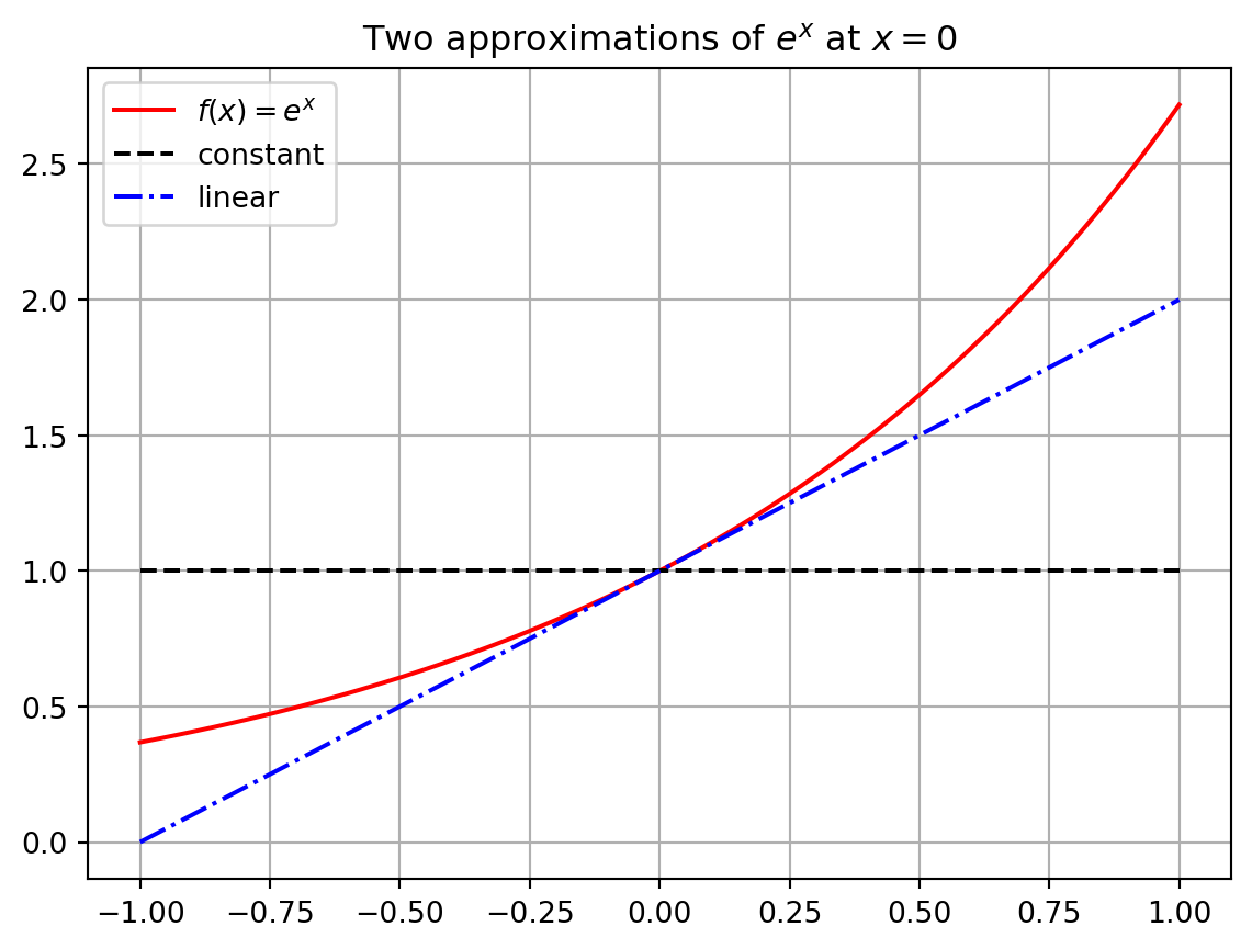
The function $g(x) = 1$ matches $f(x) = e^x$ exactly at the point $x=0$ since $f(0) = e^0 = 1$. Furthermore if $x$ is very very close to $0$ then the functions $f(x)$ and $g(x)$ are really close to each other. Hence we could say that $g(x) = 1$ is an approximation of the function $f(x) = e^x$ for values of $x$ very very close to $x=0$. Admittedly, though, it is probably pretty clear that this is a horrible approximation for any $x$ just a little bit away from $x=0$.
Let us get a better approximation. What if we insist that our approximation $g(x)$ matches $f(x) = e^x$ exactly at $x=0$ and ALSO has exactly the same first derivative as $f(x)$ at $x=0$.
1. What is the first derivative of $f(x)$?
2. What is $f'(0)$?
3. Use the point-slope form of a line to write the equation of the function $g(x)$ that goes through the point $(0,f(0))$ and has slope $f'(0)$. Recall from algebra that the point-slope form of a line is $y = f(x_0) + m(x-x_0).$ In this case we are taking $x_0 = 0$ so we are using the formula $g(x) = f(0) + f'(0) (x-0)$ to get the equation of the line.
Write Python code to build a plot like Figure 3.1. This plot shows $f(x) = e^x$, our first approximation $g(x) = 1$ and our second approximation $g(x) = 1+x$. You may want to refer back to Exercise 1.18 in the Python chapter.

Figure 3.1: The first two polynomial approximations of the exponential function.

Exercise 3.5 Let us extend the idea from the previous problem to much better approximations of the function $f(x) = e^x$.

Let us build a function $g(x)$ that matches $f(x)$ exactly at $x=0$, has exactly the same first derivative as $f(x)$ at $x=0$, AND has exactly the same second derivative as $f(x)$ at $x=0$. To do this we will use a quadratic function. For a quadratic approximation of a function we just take a slight extension to the point-slope form of a line and use the equation \[\begin{equation} y = f(x_0) + f'(x_0) (x-x_0) + \frac{f''(x_0)}{2} (x-x_0)^2. \end{equation}\] In this case we are using $x_0 = 0$ so the quadratic approximation function looks like \[\begin{equation} y = f(0) + f'(0) x + \frac{f''(0)}{2} x^2. \end{equation}\]
1. Find the quadratic approximation for $f(x) = e^x$.
2. How do you know that this function matches $f(x)$ in all of the ways described above at $x=0$?
3. Add your new function to the plot you created in the previous problem.
Let us keep going!! Next we will do a cubic approximation. A cubic approximation takes the form \[\begin{equation} y = f(x_0) + f'(0) (x-x_0) + \frac{f''(0)}{2}(x-x_0)^2 + \frac{f'''(0)}{3!}(x-x_0)^3 \end{equation}\]
1. Find the cubic approximation for $f(x) = e^x$.
2. How do we know that this function matches the first, second, and third derivatives of $f(x)$ at $x=0$?
3. Add your function to the plot.
4. Pause and think: What’s the deal with the $3!$ on the cubic term?
Your turn: Build the next several approximations of $f(x) = e^x$ at $x=0$. Add these plots to the plot that we have been building all along.

Exercise 3.6 🎓 Use the functions that you have built to approximate $\frac{1}{e} = e^{-1}$. Check the accuracy of your answer using np.exp(-1) in Python.

What we have been exploring so far in this section is the Taylor Series of a function.

Definition 3.1 (Taylor Series) If $f(x)$ is an infinitely differentiable function at the point $x_0$ then \[\begin{equation} f(x) = f(x_0) + f'(x_0)(x-x_0) + \frac{f''(x_0)}{2}(x-x_0)^2 + \cdots \frac{f^{(n)}(x_0)}{n!}(x-x_0)^n + \cdots \end{equation}\] for any reasonably small interval around $x_0$. The infinite polynomial expansion is called the Taylor Series of the function $f(x)$. Taylor Series are named for the mathematician Brook Taylor.

The Taylor Series of a function is often written with summation notation as \[\begin{equation} f(x) = \sum_{k=0}^\infty \frac{f^{(k)}(x_0)}{k!} (x-x_0)^k. \end{equation}\] Do not let the notation scare you. In a Taylor Series you are just saying: give me a function that

matches $f(x)$ at $x=x_0$ exactly,
matches $f'(x)$ at $x=x_0$ exactly,
matches $f''(x)$ at $x=x_0$ exactly,
matches $f'''(x)$ at $x=x_0$ exactly,
etc.

(Take a moment and make sure that the summation notation makes sense to you.)

Moreover, Taylor Series are built out of the easiest types of functions: polynomials. Computers are rather good at doing computations with addition, subtraction, multiplication, division, and integer exponents, so Taylor Series are a natural way to express functions in a computer. The down side is that we can only get true equality in the Taylor Series if we have infinitely many terms in the series. A computer cannot do infinitely many computations. So, in practice, we truncate Taylor Series after many terms and think of the new polynomial function as being close enough to the actual function so far as we do not stray too far from the anchor $x_0$.

Exercise 3.7 Do all of the calculations to show that the Taylor Series centred at $x_0 = 0$ for the function $f(x) = \sin(x)$ is indeed \[\begin{equation} \sin(x) = x - \frac{x^3}{3!} + \frac{x^5}{5!} - \frac{x^7}{7!} + \cdots \end{equation}\]

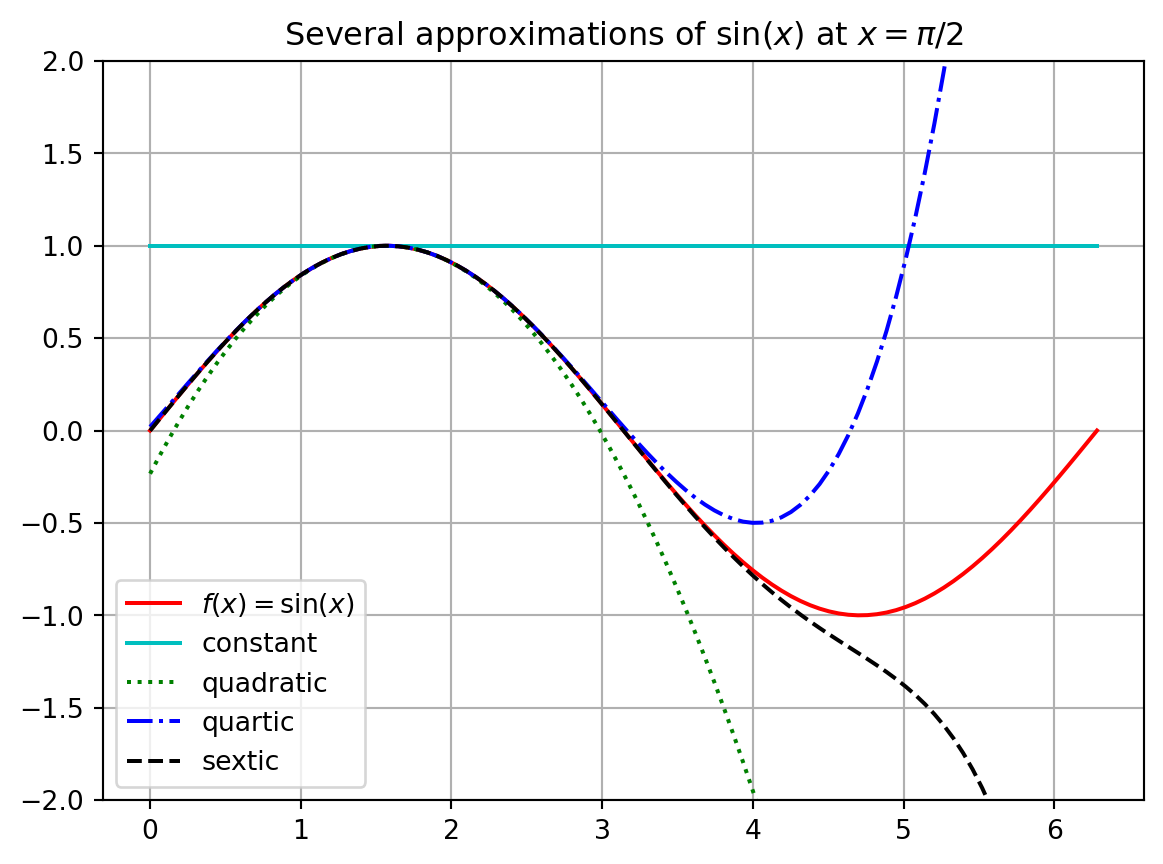
Exercise 3.8 Let us compute a few Taylor Series that are not centred at $x_0 = 0$. For example, let us approximate the function $f(x) = \sin(x)$ near $x_0 = \frac{\pi}{2}$. Near the point $x_0 = \frac{\pi}{2}$, the Taylor Series approximation will take the form \[\begin{equation} f(x) = f\left( \frac{\pi}{2} \right) + f'\left( \frac{\pi}{2} \right)\left( x - \frac{\pi}{2} \right) + \frac{f''\left( \frac{\pi}{2} \right)}{2!}\left( x - \frac{\pi}{2} \right)^2 + \frac{f'''\left( \frac{\pi}{2} \right)}{3!}\left( x - \frac{\pi}{2} \right)^3 + \cdots \end{equation}\]

Write the first several terms of the Taylor Series for $f(x) = \sin(x)$ centred at $x_0 = \frac{\pi}{2}$. Then write Python code to build the plot below showing successive approximations for $f(x) = \sin(x)$ centred at $\pi/2$.

Figure 3.2: Taylor series approximation of the sine function.

Exercise 3.9 🎓 Repeat the previous exercise for the function \[ f(x) = \log(x) \text{ centered at } x_0 = 1. \] Use this to give an approximate value for $\log(1.1)$.

Example 3.1 Let us conclude this brief section by examining an interesting example. Consider the function \[\begin{equation} f(x) = \frac{1}{1-x}. \end{equation}\] If we build a Taylor Series centred at $x_0 = 0$ it is not too hard to show that we get \[\begin{equation} f(x) = 1 + x + x^2 + x^3 + x^4 + x^5 + \cdots \end{equation}\] (you should stop now and verify this!). However, if we plot the function $f(x)$ along with several successive approximations for $f(x)$ we find that beyond $x=1$ we do not get the correct behaviour of the function (see Figure 3.3). More specifically, we cannot get the Taylor Series to change behaviour across the vertical asymptote of the function at $x=1$. This example is meant to point out the fact that a Taylor Series will only ever make sense near the point at which you centre the expansion. For the function $f(x) = \frac{1}{1-x}$ centred at $x_0 = 0$ we can only get good approximations within the interval $x \in (-1,1)$ and no further.

Code

import numpy as np
import math as ma
import matplotlib.pyplot as plt

# build the x and y values
x = np.linspace(-1,2,101)
y0 = 1/(1-x)
y1 = 1 + 0*x
y2 = 1 + x
y3 = y2 + x**2
y4 = y3 + x**3 + x**4 + x**5 + x**6 + x**7 + x**8

# plot each of the functions 
plt.plot(x, y0, 'r-', label=r"$f(x)=1/(1-x)$")
plt.plot(x, y1, 'c-', label=r"constant")
plt.plot(x, y2, 'g:', label=r"linear")
plt.plot(x, y3, 'b-.', label=r"quadratic")
plt.plot(x, y4, 'k--', label=r"8th order")

# set limits on the y axis
plt.ylim(-3,5)

# put in a grid, legend, title, and axis labels
plt.grid()
plt.legend()
plt.title(r"Taylor approximations of $f(x)=\frac{1}{1-x}$ around $x=0$")
plt.show()

Figure 3.3: Several Taylor Series approximations of the function $f(x) = 1/(1-x)$.

In the previous example we saw that we cannot always get approximations from Taylor Series that are good everywhere. For every Taylor Series there is a domain of convergence where the Taylor Series actually makes sense and gives good approximations. While it is beyond the scope of this section to give all of the details for finding the domain of convergence for a Taylor Series, a good heuristic is to observe that a Taylor Series will only give reasonable approximations of a function from the centre of the series to the nearest asymptote. The domain of convergence is typically symmetric about the centre as well. For example:

If we were to build a Taylor Series approximation for the function $f(x) = \log(x)$ centred at the point $x_0 = 1$ then the domain of convergence should be $x \in (0,2)$ since there is a vertical asymptote for the natural logarithm function at $x=0$.
If we were to build a Taylor Series approximation for the function $f(x) = \frac{5}{2x-3}$ centred at the point $x_0 = 4$ then the domain of convergence should be $x \in (1.5, 6.5)$ since there is a vertical asymptote at $x=1.5$ and the distance from $x_0 = 4$ to $x=1.5$ is 2.5 units.
If we were to build a Taylor Series approximation for the function $f(x) = \frac{1}{1+x^2}$ centred at the point $x_0 = 0$ then the domain of convergence should be $x \in (-1,1)$. This may seem quite odd (and perhaps quite surprising!) but let us think about where the nearest asymptote might be. To find the asymptote we need to solve $1+x^2 = 0$ but this gives us the values $x = \pm i$. In the complex plane, the numbers $i$ and $-i$ are 1 unit away from $x_0 = 0$, so the “asymptote” is not visible in a real-valued plot but it is still only one unit away. Hence the domain of convergence is $x \in (-1,1)$. You may want to pause now and build some plots to show yourself that this indeed appears to be true.

Of course you learned all this and more in your first-year Calculus but I hope it was fun to now rediscover these things yourself. In your Calculus module it was probably not stressed how fundamental Taylor series are to doing numerical computations.

3.2 Truncation Error

The great thing about Taylor Series is that they allow for the representation of potentially very complicated functions as polynomials – and polynomials are easily dealt with on a computer since they involve only addition, subtraction, multiplication, division, and integer powers. The down side is that the order of the polynomial is infinite. Hence, every time we use a Taylor series on a computer, what we are actually going to be using is a Truncated Taylor Series where we only take a finite number of terms. The idea here is simple in principle:

If a function $f(x)$ has a Taylor Series representation it can be written as an infinite sum.
Computers cannot do infinite sums.
So stop the sum at some point $n$ and throw away the rest of the infinite sum.
Now $f(x)$ is approximated by some finite sum so long as you stay pretty close to $x = x_0$,
and everything that we just chopped off of the end is called the remainder for the finite sum.

Let us be a bit more concrete about it. The Taylor Series for $f(x) = e^x$ centred at $x_0 = 0$ is \[\begin{equation} e^x = 1 + x + \frac{x^2}{2!} + \frac{x^3}{3!} + \frac{x^4}{4!} + \cdots. \end{equation}\]

$0^{th}$ Order Approximation of $f(x) = e^x$:: If we want to use a zeroth-order (constant) approximation $f_0(x)$ of the function $f(x) = e^x$ then we only take the first term in the Taylor Series and the rest is not used for the approximation \[\begin{equation} e^x = \underbrace{1}_{\text{$0^{th}$ order approximation}} + \underbrace{x + \frac{x^2}{2!} + \frac{x^3}{3!} + \frac{x^4}{4!} + \cdots}_{\text{remainder}}. \end{equation}\] Therefore we would approximate $e^x$ as $e^x \approx 1=f_0(x)$ for values of $x$ that are close to $x_0 = 0$. Furthermore, for small values of $x$ that are close to $x_0 = 0$ the largest term in the remainder is $x$ (since for small values of $x$ like 0.01, $x^2$ will be even smaller, $x^3$ even smaller than that, etc). This means that if we use a $0^{th}$ order approximation for $e^x$ then we expect our error to be about the same size as $x$. It is common to then rewrite the truncated Taylor Series as \[\begin{equation} \text{$0^{th}$ order approximation: } e^x \approx 1 + \mathcal{O}(x) \end{equation}\] where $\mathcal{O}(x)$ (read “Big-O of $x$”) tells us that the expected error for approximations close to $x_0 = 0$ is about the same size as $x$.
$1^{st}$ Order Approximation of $f(x) = e^x$:: If we want to use a first-order (linear) approximation $f_1(x)$ of the function $f(x) = e^x$ then we gather the $0^{th}$ order and $1^{st}$ order terms together as our approximation and the rest is the remainder \[\begin{equation} e^x = \underbrace{1 + x}_{\text{$1^{st}$ order approximation}} + \underbrace{\frac{x^2}{2!} + \frac{x^3}{3!} + \frac{x^4}{4!} + \cdots}_{\text{remainder}}. \end{equation}\] Therefore we would approximate $e^x$ as $e^x \approx 1+x=f_1(x)$ for values of $x$ that are close to $x_0 = 0$. Furthermore, for values of $x$ very close to $x_0 = 0$ the largest term in the remainder is the $x^2$ term. Using Big-O notation we can write the approximation as \[\begin{equation} \text{$1^{st}$ order approximation: } e^x \approx 1 + x + \mathcal{O}(x^2). \end{equation}\] Notice that we do not explicitly say what the coefficient is for the $x^2$ term. Instead we are just saying that using the linear function $y=1+x$ to approximate $e^x$ for values of $x$ near $x_0=0$ will result in errors that are of the order of $x^2$.
$2^{nd}$ Order Approximation of $f(x) = e^x$:: If we want to use a second-order (quadratic) approximation $f_2(x)$ of the function of $f(x) = e^x$ then we gather the $0^{th}$ order, $1^{st}$ order, and $2^{nd}$ order terms together as our approximation and the rest is the remainder \[\begin{equation} e^x = \underbrace{1 + x + \frac{x^2}{2!}}_{\text{$2^{nd}$ order approximation}} + \underbrace{\frac{x^3}{3!} + \frac{x^4}{4!} + \cdots}_{\text{remainder}}. \end{equation}\] Therefore we would approximate $e^x$ as $e^x \approx 1+x+\frac{x^2}{2}=f_2(x)$ for values of $x$ that are close to $x_0 = 0$. Furthermore, for values of $x$ very close to $x_0 = 0$ the largest term in the remainder is the $x^3$ term. Using Big-O notation we can write the approximation as \[\begin{equation} \text{$2^{nd}$ order approximation: } e^x \approx 1 + x + \frac{x^2}{2} + \mathcal{O}(x^3). \end{equation}\] Again notice that we do not explicitly say what the coefficient is for the $x^3$ term. Instead we are just saying that using the quadratic function $y=1+x+\frac{x^2}{2}$ to approximate $e^x$ for values of $x$ near $x_0=0$ will result in errors that are of the order of $x^3$.

Keep in mind that this sort of analysis is only good for values of $x$ that are very close to the centre of the Taylor Series. If you are making approximations that are too far away then all bets are off.

For the function $f(x) = e^x$ the idea of approximating the amount of approximation error by truncating the Taylor Series is relatively straight forward: if we want an $n^{th}$ order polynomial approximation $f_n(x)$ of the function of $f(x)=e^x$ near $x_0 = 0$ then \[\begin{equation} e^x = 1 + x + \frac{x^2}{2!} + \frac{x^3}{3!} + \frac{x^4}{4!} + \cdots + \frac{x^n}{n!} + \mathcal{O}(x^{n+1}), \end{equation}\] meaning that we expect the error to be of the order of $x^{n+1}$.

Exercise 3.10 🎓 Now make the previous discussion a bit more concrete. You know the Taylor Series for $f(x) = e^x$ around $x=0$ quite well at this point so use it to approximate the values of $f(0.1) = e^{0.1}$ and $f(0.2)=e^{0.2}$ by truncating the Taylor series at different orders. Because $x=0.1$ and $x=0.2$ are pretty close to the centre of the Taylor Series $x_0 = 0$, this sort of approximation is reasonable.

Then compare your approximate values to Python’s values $f(0.1)=e^{0.1} \approx$ np.exp(0.1) $=1.1051709180756477$ and $f(0.2)=e^{0.2} \approx$ np.exp(0.2) $=1.2214027581601699$ to calculate the truncation errors $\epsilon_n(0.1)=|f(0.1)-f_n(0.1)|$ and $\epsilon_n(0.2)=|f(0.2)-f_n(0.2)|$.

Fill in the blanks in the table. If you want to create the table in your jupyter notebook, you can use Pandas as described in Section 1.6. Alternatively feel free to use a spreadsheet instead of using Python.

Order $n$	$f_n(0.1)$	$\epsilon_n(0.1)=\|f(0.1)-f_n(0.1)\|$	$f_n(0.2)$	$\epsilon_n(0.2)=\|f(0.2)-f_n(0.2)\|$
0	1	1.051709e-01	1	2.214028e-01
1	1.1	5.170918e-03	1.2
2	1.105
3
4
5

You will find that, as expected, the truncation errors $\epsilon_n(x)$ decrease with $n$ but increase with $x$.

Exercise 3.11 To investigate the dependence of the truncation error $\epsilon_n(x)$ on $n$ and $x$ a bit more, add an extra column to the table from the previous exercise with the ratio $\epsilon_n(0.2) / \epsilon_n(0.1)$.

Order $n$	$\epsilon_n(0.1)$	$\epsilon_n(0.2)$	$\epsilon_n(0.2) / \epsilon_n(0.1)$
0	1.051709e-01	2.214028e-01	2.105171
1	5.170918e-03
2
3
4
5

Formulate a conjecture about how $\epsilon_n$ changes as $x$ changes.

Exercise 3.12 To test your conjecture, examine the truncation error for the sine function near $x_0 = 0$. You know that the sine function has the Taylor Series centred at $x_0 = 0$ as \[\begin{equation} f(x) = \sin(x) = x - \frac{x^3}{3!} + \frac{x^5}{5!} - \frac{x^7}{7!} + \cdots. \end{equation}\] So there are only approximations of odd order. Use the truncated Taylor series to approximate $f(0.1)=\sin(0.1)$ and $f(0.2)=\sin(0.2)$ and use Python’s values np.sin(0.1) and np.sin(0.2) to calculate the truncation errors $\epsilon_n(0.1)=|f(0.1)-f_n(0.1)|$ and $\epsilon_n(0.2)=|f(0.2)-f_n(0.2)|$.

Complete the following table:

Order $n$	$\epsilon_n(0.1)$	$\epsilon_n(0.2)$
1	1.665834e-04	1.330669e-03
3	8.331349e-08	2.664128e-06
5	1.983852e-11
7
9

The entry in the last row of the table will almost certainly not agree with your conjecture. That is okay! That discrepancy has a different explanation. Can you figure out what it is? Hint: does np.sin(x) give you the exact value of $\sin(x)$?

Exercise 3.13 🎓 Perform another check of your conjecture by approximating $\log(1.02)$ and $\log(1.1)$ from truncations of the Taylor series around $x=1$: \[ \log(1+x) = x - \frac{x^2}{2} + \frac{x^3}{3} - \frac{x^4}{4} + \frac{x^5}{5} - \cdots. \] If you are using Python then use np.log1p(x) to calculate $\log(1+x)$.

Exercise 3.14 Write down your observations about how the truncation error at order $n$ changes as $x$ changes. Explain this in terms of the form of the remainder of the truncated Taylor series.

3.3 Problems

Exercise 3.15 Find the Taylor Series for $f(x) = \frac{1}{\log(x)}$ centred at the point $x_0 = e$. Then use the Taylor Series to approximate the number $\frac{1}{\log(3)}$ to 4 decimal places.

Exercise 3.16 In this problem we will use Taylor Series to build approximations for the irrational number $\pi$.

Write the Taylor series centred at $x_0=0$ for the function \[\begin{equation} f(x) = \frac{1}{1+x}. \end{equation}\]
Now we want to get the Taylor Series for the function $g(x) = \frac{1}{1+x^2}$. It would be quite time consuming to take all of the necessary derivatives to get this Taylor Series. Instead we will use our answer from part (a) of this problem to shortcut the whole process.
1. Substitute $x^2$ for every $x$ in the Taylor Series for $f(x) = \frac{1}{1+x}$.
2. Make a few plots to verify that we indeed now have a Taylor Series for the function $g(x) = \frac{1}{1+x^2}$.
Recall from Calculus that \[\begin{equation} \int \frac{1}{1+x^2} dx = \arctan(x). \end{equation}\] Hence, if we integrate each term of the Taylor Series that results from part (b) we should have a Taylor Series for $\arctan(x)$.¹
Now recall the following from Calculus:

$\tan(\pi/4) = 1$
so $\arctan(1) = \pi/4$
and therefore $\pi = 4\arctan(1)$.

Let us use these facts along with the Taylor Series for $\arctan(x)$ to approximate $\pi$: we can just plug in $x=1$ to the series, add up a bunch of terms, and then multiply by 4. Write a loop in Python that builds successively better and better approximations of $\pi$. Stop the loop when you have an approximation that is correct to 6 decimal places.

Exercise 3.17 In this problem we will prove the famous (and the author’s favourite) formula \[\begin{equation} e^{i\theta} = \cos(\theta) + i \sin(\theta). \end{equation}\] This is known as Euler’s formula after the famous mathematician Leonard Euler. Show all of your work for the following tasks.

Write the Taylor series for the functions $e^x$, $\sin(x)$, and $\cos(x)$.
Replace $x$ with $i\theta$ in the Taylor expansion of $e^x$. Recall that $i = \sqrt{-1}$ so $i^2 = -1$, $i^3 = -i$, and $i^4 = 1$. Simplify all of the powers of $i\theta$ that arise in the Taylor expansion. I will get you started: \[\begin{equation} \begin{aligned} e^x &= 1 + x + \frac{x^2}{2} + \frac{x^3}{3!} + \frac{x^4}{4!} + \frac{x^5}{5!} + \cdots \\ e^{i\theta} &= 1 + (i\theta) + \frac{(i\theta)^2}{2!} + \frac{(i\theta)^3}{3!} + \frac{(i\theta)^4}{4!} + \frac{(i\theta)^5}{5!} + \cdots \\ &= 1 + i\theta + i^2 \frac{\theta^2}{2!} + i^3 \frac{\theta^3}{3!} + i^4 \frac{\theta^4}{4!} + i^5 \frac{\theta^5}{5!} + \cdots \\ &= \ldots \text{ keep simplifying ... } \ldots \end{aligned} \end{equation}\]
Gather all of the real terms and all of the imaginary terms together. Factor the $i$ out of the imaginary terms. What do you notice?
Use your result from part (c) to prove that $e^{i\pi} + 1 = 0$.

Exercise 3.18 In physics, the relativistic energy of an object is defined as \[\begin{equation} E_{rel} = \gamma mc^2 \end{equation}\] where \[\begin{equation} \gamma = \frac{1}{\sqrt{1 - \frac{v^2}{c^2}}}. \end{equation}\] In these equations, $m$ is the mass of the object, $c$ is the speed of light ($c \approx 3 \times 10^8$m/s), and $v$ is the velocity of the object. For an object of fixed mass (m) we can expand the Taylor Series centred at $v=0$ for $E_{rel}$ to get \[\begin{equation} E_{rel} = mc^2 + \frac{1}{2} mv^2 + \frac{3}{8} \frac{mv^4}{c^2} + \frac{5}{16} \frac{mv^6}{c^4} + \cdots. \end{equation}\]

What do we recover if we consider an object with zero velocity?
Why might it be completely reasonable to only use the quadratic approximation \[\begin{equation} E_{rel} = mc^2 + \frac{1}{2} mv^2 \end{equation}\] for the relativistic energy equation?²
(some physics knowledge required) What do you notice about the second term in the Taylor Series approximation of the relativistic energy function?
Show all of the work to derive the Taylor Series centred at $v = 0$ given above.

There are many reasons why integrating an infinite series term by term should give you a moment of pause. For the sake of this problem we are doing this operation a little blindly, but in reality we should have verified that the infinite series actually converges uniformly.↩︎
This is something that people in physics and engineering do all the time – there is some complicated nonlinear relationship that they wish to use, but the first few terms of the Taylor Series captures almost all of the behaviour since the higher-order terms are very very small.↩︎

Order \(n\)	\(\epsilon_n(0.1)\)	\(\epsilon_n(0.2)\)	\(\epsilon_n(0.2) / \epsilon_n(0.1)\)
0	1.051709e-01	2.214028e-01	2.105171
1	5.170918e-03
2
3
4
5