def bisection_with_error_tracking(f, x_exact, a, b, tol):
"""
Implements the bisection method and tracks absolute error at each iteration.
Args:
f (callable): Function for which to find the root
x_exact (float): The exact root of the function
a (float): Left endpoint of initial interval
b (float): Right endpoint of initial interval
tol (float): Tolerance for stopping criterion
Returns:
list: List of absolute errors between approximate and exact solution at each iteration
"""
errors = []
while (b - a) / 2.0 > tol:
midpoint = (a + b) / 2.0
if f(midpoint) == 0:
break
elif f(a) * f(midpoint) < 0:
b = midpoint
else:
a = midpoint
error = abs(midpoint - x_exact)
errors.append(error)
return errors4 Non-linear Equations
Success is the sum of small efforts, repeated day in and day out.
–Zeno of Elea
4.1 Introduction to Numerical Root Finding
In this chapter we want to solve equations using a computer. The goal of equation solving is to find the value of the independent variable which makes the equation true. These are the sorts of equations that you learned to solve at school. For a very simple example, solve for \(x\) if \(x+5 = 2x- 3\). Or, for another example, the equation \(x^2+x=2x - 7\) is an equation that could be solved with the quadratic formula. The equation \(\sin(x) = \frac{\sqrt{2}}{2}\) is an equation which can be solved using some knowledge of trigonometry. The topic of Numerical Root Finding really boils down to approximating the solutions to equations without using all of the by-hand techniques that you learned in high school. The down side to everything that we are about to do is that our answers are only ever going to be approximations.
The fact that we will only ever get approximate answers begs the question: why would we want to do numerical algebra if by-hand techniques exist? The answers are relatively simple:
Most equations do not lend themselves to by-hand solutions. The reason you may not have noticed that is that we tend to show you only nice equations that arise in often very simplified situations. When equations arise naturally they are often not nice.
By-hand algebra is often very challenging, quite time consuming, and error prone. You will find that the numerical techniques are quite elegant, work very quickly, and require very little overhead to actually implement and verify.
Let us first take a look at equations in a more abstract way. Consider the equation \(\ell(x) = r(x)\) where \(\ell(x)\) and \(r(x)\) stand for left-hand and right-hand expressions respectively. To begin solving this equation we can first rewrite it by subtracting the right-hand side from the left to get \[\begin{equation} \ell(x) - r(x) = 0. \end{equation}\] Hence, we can define a function \(f(x)\) as \(f(x)=\ell(x)-r(x)\) and observe that every equation can be written as: \[\begin{equation} \text{ Find } x \text{ such that } f(x) = 0. \end{equation}\] This gives us a common language for which to frame all of our numerical algorithms. An \(x\) where \(f(x)=0\) is called a root of \(f\) and thus we have seen that solving an equation is always a root finding problem.
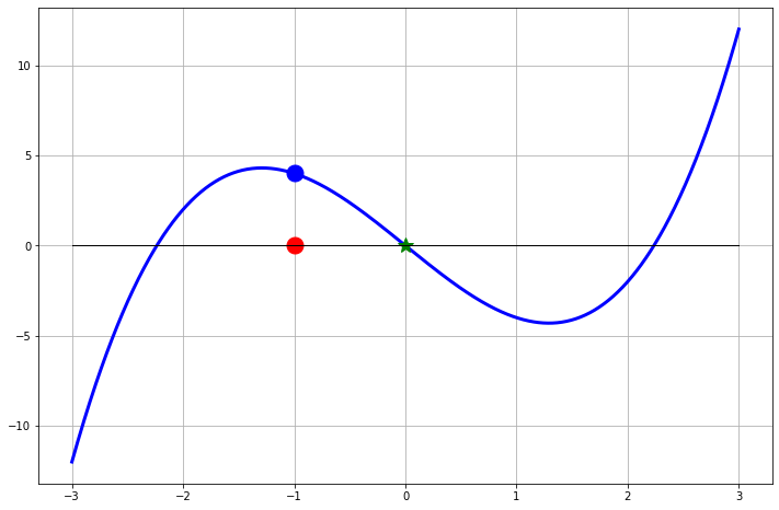
For example, if we want to solve the equation \(3\sin(x) + 9 = x^2 - \cos(x)\) then this is the same as solving \((3\sin(x) + 9 ) - (x^2 - \cos(x)) = 0\). We illustrate this idea in Figure 4.1. You should pause and notice that there is no way that you are going to apply by-hand techniques from algebra to solve this equation … an approximate answer is pretty much our only hope.
Code
import numpy as np
import matplotlib.pyplot as plt
x = np.linspace(-4,4, 100)
l = 3 * np.sin(x) + 9
r = x**2 - np.cos(x)

fig, axes = plt.subplots(nrows = 1, ncols = 2)

axes[0].plot(x, l, 'b-.', label=r"$3\sin(x)+9$")
axes[0].plot(x, r, 'r-', label=r"$x^2-\cos(x)$")
axes[0].grid()
axes[0].legend()
axes[0].set_title(r"$3\sin(x)+9 = x^2-\cos(x)$")

axes[1].plot(x, l-r, 'g:', label=r"(3\sin(x)+9) - (x^2-\cos(x))")
axes[1].plot(x, np.zeros(100), 'k-')
axes[1].grid()
axes[1].legend()
axes[1].set_title(r"$(3\sin(x)+9) - (x^2-\cos(x))=0$")

fig.tight_layout()
plt.show()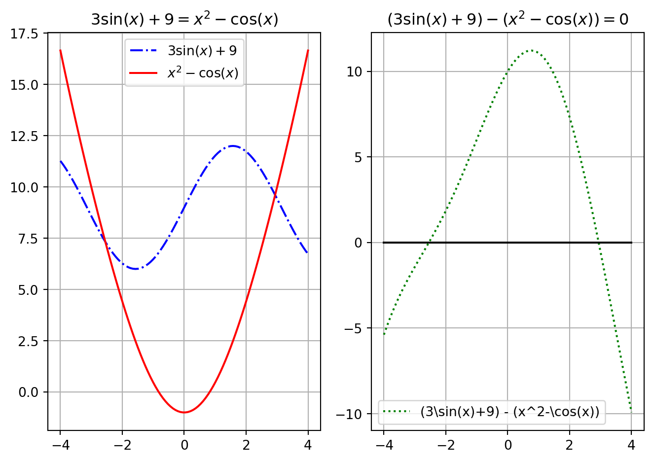
On the left-hand side of Figure 4.1 we see the solutions as the intersections of the graph of \(3\sin(x) + 9\) with the graph of \(x^2 - \cos(x)\), and on the right-hand side we see the solutions as the intersections of the graph of \(\left( 3\sin(x)+9 \right) - \left( x^2 - \cos(x) \right)\) with the \(x\) axis. From either plot we can read off the approximate solutions: \(x_1 \approx -2.55\) and \(x_2 \approx 2.88\). Figure 4.1 should demonstrate what we mean when we say that solving equations of the form \(\ell(x) = r(x)\) will give the same answer as finding the roots of \(f(x) = \ell(x)-r(x)\).
We now have one way to view every equation-solving problem. As we will see in this chapter, if \(f(x)\) has certain properties then different numerical techniques for solving the equation will apply – and some will be much faster and more accurate than others. In the following sections you will develop several different techniques for solving equations of the form \(f(x) = 0\). You will start with the simplest techniques to implement and then move to the more powerful techniques that use some ideas from Calculus to understand and analyse. Throughout this chapter you will also work to quantify the amount of error that one makes when using these techniques.
4.2 The Bisection Method
4.2.1 Intuition
Exercise 4.1 A friend tells you that she is thinking of a number between 1 and 100. She will allow you multiple guesses with some feedback for where the mystery number falls. How do you systematically go about guessing the mystery number? Is there an optimal strategy?
For example, the conversation might go like this.
- Sally: I am thinking of a number between 1 and 100.
- Joe: Is it 35?
- Sally: No, 35 is too low.
- Joe: Is it 99?
- Sally: No, 99 is too high.
- …
Exercise 4.2 Imagine that Sally likes to formulate her answer not in the form “\(x\) is too small” or “\(x\) is too large” but in the form “\(f(x)\) is positive” or “\(f(x)\) is negative”. If she uses \(f(x) = x-x_0\), where \(x_0\) is Sally’s chosen number then her new answers contain exactly the same information as her previous answers? Can you now explain how Sally’s game is a root finding game?
Exercise 4.3 Now go and play the game with other functions \(f(x)\). Choose someone from your group to be Sally and someone else to be Joe. Sally can choose a continuous function and Joe needs to guess its root. Does your strategy still allow Joe to find the root of \(f(x)\) at least approximately? When should the game stop? Does Sally need to give Joe some extra information to give him a fighting chance?
Exercise 4.4 Was it necessary to say that Sally’s function was continuous? Does your strategy work if the function is not continuous.
Now let us get to the maths. We will start the mathematical discussion with a theorem from Calculus.
Theorem 4.1 (The Intermediate Value Theorem (IVT)) If \(f(x)\) is a continuous function on the closed interval \([a,b]\) and \(y_*\) lies between \(f(a)\) and \(f(b)\), then there exists some point \(x_* \in [a,b]\) such that \(f(x_*) = y_*\).
Exercise 4.5 Draw a picture of what the intermediate value theorem says graphically.
Exercise 4.6 If \(y_*=0\) the Intermediate Value Theorem gives us important information about solving equations. What does it tell us?
Corollary 4.1 If \(f(x)\) is a continuous function on the closed interval \([a,b]\) and if \(f(a)\) and \(f(b)\) have opposite signs then from the Intermediate Value Theorem we know that there exists some point \(x_* \in [a,b]\) such that ____.
Exercise 4.7 Fill in the blank in the previous corollary and then draw several pictures that indicate why this might be true for continuous functions.
The Intermediate Value Theorem (IVT) and its corollary are existence theorems in the sense that they tell us that some point exists. The annoying thing about mathematical existence theorems is that they typically do not tell us how to find the point that is guaranteed to exist. The method that you developed in Exercise 4.1 to Exercise 4.3 gives one possible way to find the root.
In those exercises you likely came up with an algorithm such as this:
Say we know that a continuous function has opposite signs at \(x=a\) and \(x=b\).
Guess that the root is at the midpoint \(m = \frac{a+b}{2}\).
By using the signs of the function, narrow the interval that contains the root to either \([a,m]\) or \([m,b]\).
Repeat until the interval is small enough.
Now we will turn this strategy into computer code that will simply play the game for us. But first we need to pay careful attention to some of the mathematical details.
Exercise 4.8 Where is the Intermediate Value Theorem used in the root-guessing strategy?
Exercise 4.9 Why was it important that the function \(f(x)\) is continuous when playing this root-guessing game? Provide a few sketches to demonstrate your answer.
4.2.2 Implementation
Exercise 4.10 (The Bisection Method) Goal: We want to solve the equation \(f(x) = 0\) for \(x\) assuming that the solution \(x^*\) is in the interval \([a,b]\).
The Algorithm: Assume that \(f(x)\) is continuous on the closed interval \([a,b]\). To make approximations of the solutions to the equation \(f(x) = 0\), do the following:
Check to see if \(f(a)\) and \(f(b)\) have opposite signs. You can do this taking the product of \(f(a)\) and \(f(b)\).
If \(f(a)\) and \(f(b)\) have different signs then what does the IVT tell you?
If \(f(a)\) and \(f(b)\) have the same sign then what does the IVT not tell you? What should you do in this case?
Why does the product of \(f(a)\) and \(f(b)\) tell us something about the signs of the two numbers?
Compute the midpoint of the closed interval, \(m=\frac{a+b}{2}\), and evaluate \(f(m)\).
Will \(m\) always be a better guess of the root than \(a\) or \(b\)? Why?
What should you do here if \(f(m)\) is really close to zero?
Compare the signs of \(f(a)\) versus \(f(m)\) and \(f(b)\) versus \(f(m)\).
What do you do if \(f(a)\) and \(f(m)\) have opposite signs?
What do you do if \(f(m)\) and \(f(b)\) have opposite signs?
Repeat steps 2 and 3 and stop when the interval containing the root is small enough.
Exercise 4.11 Draw a picture illustrating what the Bisection Method does to approximate a solution to an equation \(f(x) = 0\).
Exercise 4.12 We want to write a Python function for the Bisection Method. Instead of jumping straight into writing the code we should first come up with the structure of the code. It is often helpful to outline the structure as comments in your file. Use the template below and complete the comments. Note how the function starts with a so-called docstring that describes what the function does and explains the function parameters and its return value. This is standard practice and is how the help text is generated that you see when you hove over a function name in your code.
Don’t write the code yet, just complete the comments. I recommend switching off the AI for this exercise because otherwise the AI will keep already suggesting the code while you write the comments.
def Bisection(f , a , b , tol=1e-5):
    """
    Find a root of f(x) in the interval [a, b] using the bisection method
    with a given tolerance tol.

    Parameters:
        f   : function, the function for which we seek a root
        a   : float, left endpoint of the interval
        b   : float, right endpoint of the interval
        tol : float, stopping tolerance

    Returns:
        float: approximate root of f(x)
    """

    # check that a and b have opposite signs
    # if not, return an error and stop

    # calculate the midpoint m = (a+b)/2

    # start a while loop that runs while the interval is
    # larger than 2 * tol

        # if ...
        # elif ...
        # elif ...

        # Calculate midpoint of new interval

    # end the while loop
    # return the approximate root
Exercise 4.13 Now use the comments from Exercise 4.12 as structure to complete a Python function for the Bisection Method. Test your Bisection Method code on the following equations.
\(x^2 - 2 = 0\) on \(x \in [0,2]\)
\(\sin(x) + x^2 = 2\log(x) + 5\) on \(x \in [1,5]\)
\((5-x)e^{x}=5\) on \(x \in [0,5]\)
Figure 4.2 shows the bisection method in action on the equation \(x^2 - 2 = 0\).
4.2.3 Analysis
After we build any root finding algorithm we need to stop and think about how it will perform on new problems. The questions that we typically have for a root-finding algorithm are:
Will the algorithm always converge to a solution?
How fast will the algorithm converge to a solution?
Are there any pitfalls that we should be aware of when using the algorithm?
Exercise 4.14 Discussion: What must be true in order to use the bisection method?
Exercise 4.15 Discussion: Does the bisection method work if the Intermediate Value Theorem does not apply? (Hint: what does it mean for the IVT to “not apply?”)
Exercise 4.16 If there is a root of a continuous function \(f(x)\) between \(x=a\) and \(x=b\), will the bisection method always be able to find it? Why / why not?
Next we will focus on a deeper mathematical analysis that will allow us to determine exactly how fast the bisection method actually converges to within a pre-set tolerance. Work through the next problem to develop a formula that tells you exactly how many steps the bisection method needs to take before it gets close enough to the true solution.
Exercise 4.17 Let \(f(x)\) be a continuous function on the interval \([a,b]\) and assume that \(f(a) \cdot f(b) <0\). A recurring theme in Numerical Analysis is to approximate some mathematical thing to within some tolerance. For example, if we want to approximate the solution to the equation \(f(x)=0\) to within \(\varepsilon\) with the bisection method, we should be able to figure out how many steps it will take to achieve that goal.
Let us say that \(a = 3\) and \(b = 8\) and \(f(a) \cdot f(b) < 0\) for some continuous function \(f(x)\). The width of this interval is \(5\), so if we guess that the root is \(m=(3+8)/2 = 5.5\) then our error is less than \(5/2\). In the more general setting, if there is a root of a continuous function in the interval \([a,b]\) then how far off could the midpoint approximation of the root be? In other words, what is the error in using \(m=(a+b)/2\) as the approximation of the root?
The bisection method cuts the width of the interval down to a smaller size at every step. As such, the approximation error gets smaller at every step. Fill in the blanks in the following table to see the pattern in how the approximation error changes with each iteration.
| Iteration | Width of Interval | Maximal Error |
|---|---|---|
| 1 | \(|b-a|\) | \(\frac{|b-a|}{2}\) |
| 2 | \(\frac{|b-a|}{2}\) | |
| 3 | \(\frac{|b-a|}{2^2}\) | |
| \(\vdots\) | \(\vdots\) | \(\vdots\) |
| \(n\) | \(\frac{|b-a|}{2^{n-1}}\) |
- Now to the key question:
If we want to approximate the solution to the equation \(f(x)=0\) to within some tolerance \(\varepsilon\) then how many iterations of the bisection method do we need to take?
Hint: Set the \(n^{th}\) approximation error from the table equal to \(\varepsilon\). What should you solve for from there?
In Exercise 4.17 you actually proved the following theorem.
Theorem 4.2 (Convergence Rate of the Bisection Method) If \(f(x)\) is a continuous function with a root in the interval \([a,b]\) and if the bisection method is performed to find the root then:
The error between the actual root and the approximate root will decrease by a factor of 2 at every iteration.
If we want the approximate root found by the bisection method to be within a tolerance of \(\varepsilon\) then \[\begin{equation} \frac{|b-a|}{2^{n}} = \varepsilon \end{equation}\] where \(n\) is the number of iterations that it takes to achieve that tolerance.
Solving for the number \(n\) of iterations we get \[\begin{equation} n = \log_2\left( \frac{|b-a|}{\varepsilon} \right). \end{equation}\]
Rounding the value of \(n\) up to the nearest integer gives the number of iterations necessary to approximate the root to a precision less than \(\varepsilon\).
Exercise 4.18 Is it possible for a given function and a given interval that the Bisection Method converges to the root in fewer steps than what you just found in the previous problem? Explain.
Exercise 4.19 Create a second version of your Python Bisection Method function that uses a for loop that takes the exact number of steps required to guarantee that the approximation to the root lies within a requested tolerance. This should be in contrast to your first version which likely used a while loop to decide when to stop. Is there an advantage to using one of these version of the Bisection Method over the other?
The final type of analysis that we should do on the bisection method is to make plots of the error between the approximate solution that the bisection method gives you and the exact solution to the equation. This is a bit of a funny thing! Stop and think about this for a second: if you know the exact solution to the equation then why are you solving it numerically in the first place!?!? However, whenever you build an algorithm you need to test it on problems where you actually do know the answer so that you can be somewhat sure that it is not giving you nonsense. Furthermore, analysis like this tells us how fast the algorithm is expected to perform.
From Theorem 4.2 you know that the bisection method cuts the interval in half at every iteration. You proved in Exercise 4.17 that the error given by the bisection method is therefore cut in half at every iteration as well. The following example demonstrate this theorem graphically.
Example 4.1 Let us solve the very simple equation \(x^2 - 2 = 0\) for \(x\) to get the solution \(x = \sqrt{2}\) with the bisection method. Since we know the exact answer we can compare the exact answer to the value of the midpoint given at each iteration and calculate an absolute error: \[\begin{equation} \text{Absolute Error} = | \text{Approximate Solution} - \text{Exact Solution}|. \end{equation}\]
Let us write a Python function that implements the bisection method and collects the absolute errors at each iteration into a list.
We can now use this function to see the absolute error at each iteration when solving the equation \(x^2-2=0\) with the bisection method.
import numpy as np

def f(x):
    return x**2 - 2

x_exact = np.sqrt(2)

# Using the interval [1, 2] and a tolerance of 1e-7
tolerance = 1e-7
errors = bisection_with_error_tracking(f, x_exact, 1, 2, tolerance)
errors
[0.08578643762690485,
0.16421356237309515,
0.039213562373095145,
0.023286437626904855,
0.007963562373095145,
0.0076614376269048545,
0.00015106237309514547,
0.0037551876269048545,
0.0018020626269048545,
0.0008255001269048545,
0.0003372188769048545,
9.307825190485453e-05,
2.8992060595145475e-05,
3.2043095654854525e-05,
1.5255175298545254e-06,
1.3733271532645475e-05,
6.103877001395475e-06,
2.2891797357704746e-06,
3.818311029579746e-07,
5.718432134482754e-07,
9.500605524515038e-08,
1.4341252385641212e-07,
2.4203234305630872e-08]Next we write a function to plot the absolute error on the vertical axis and the iteration number on the horizontal axis. We get Figure 4.3. As expected, the absolute error follows an exponentially decreasing trend. Notice that it is not a completely smooth curve since we will have some jumps in the accuracy just due to the fact that sometimes the root will be near the midpoint of the interval and sometimes it will not be.
import matplotlib.pyplot as plt
def plot_errors(errors):
    """
    Plot the absolute errors.

    Args:
        errors (list): List of absolute errors
    """
    # Creating the x values for the plot (iterations)
    iterations = np.arange(len(errors))

    # Plotting the errors
    plt.scatter(iterations, errors, label='Error per Iteration')

    plt.xlabel('Iteration')
    plt.ylabel('Absolute Error')
    plt.title('Absolute Error in Each Iteration')
    plt.legend()
    plt.show()

plot_errors(errors)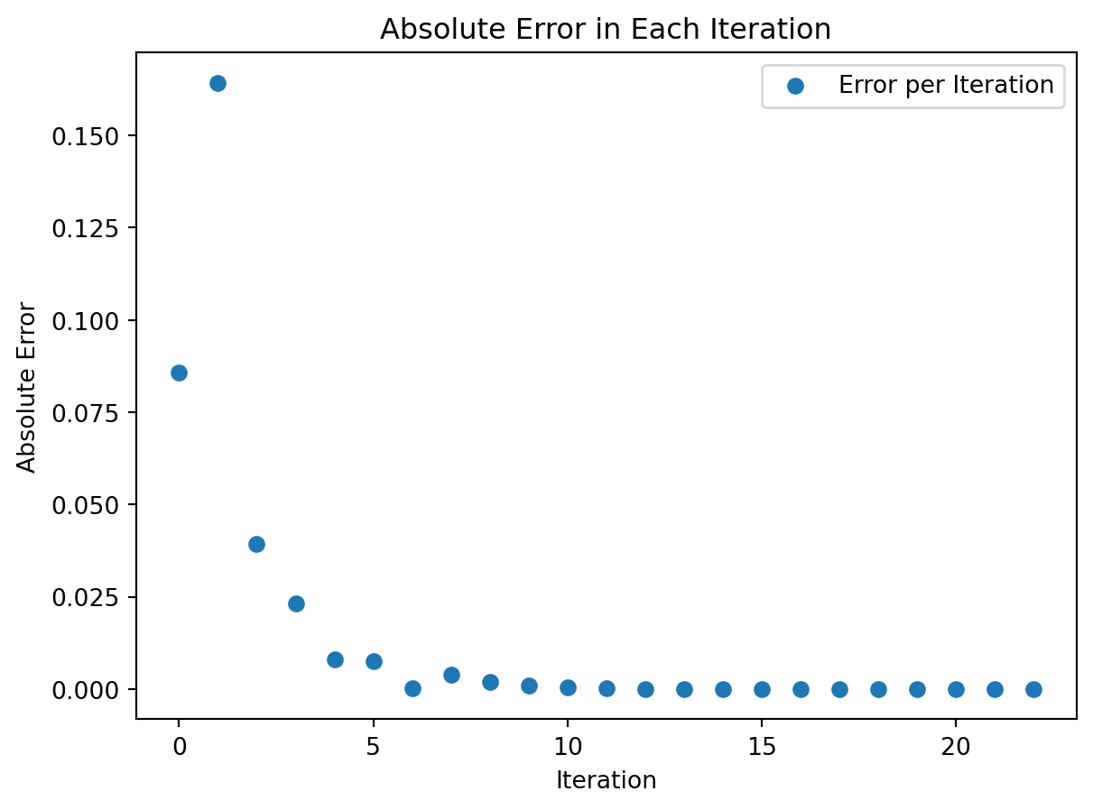
Without Theorem 4.2 it would be rather hard to tell what the exact behaviour is in the exponential plot above. We know from Theorem 4.2 that the error will divide by 2 at every step, so if we instead plot the base-2 logarithm of the absolute error against the iteration number we should see a linear trend as shown in Figure 4.4.
def plot_log_errors(errors):
    """
    Plot the base-2 logarithm of absolute errors and a best fit line.

    Args:
        errors (list): List of absolute errors
    """
    # Convert errors to base 2 logarithm
    log_errors = np.log2(errors)
    # Creating the x values for the plot (iterations)
    iterations = np.arange(len(log_errors))

    # Plotting the errors
    plt.scatter(iterations, log_errors, label='Log Error per Iteration')

    # Determine slope and intercept of the best-fit straight line
    slope, intercept = np.polyfit(iterations, log_errors, deg=1)
    best_fit_line = slope * iterations + intercept
    # Plot the best-fit line
    plt.plot(iterations, best_fit_line, label='Best Fit Line', color='red')

    plt.xlabel('Iteration')
    plt.ylabel('Base 2 Log of Absolute Error')
    plt.title('Absolute Error in Each Iteration')
    plt.legend()
    plt.show()

plot_log_errors(errors)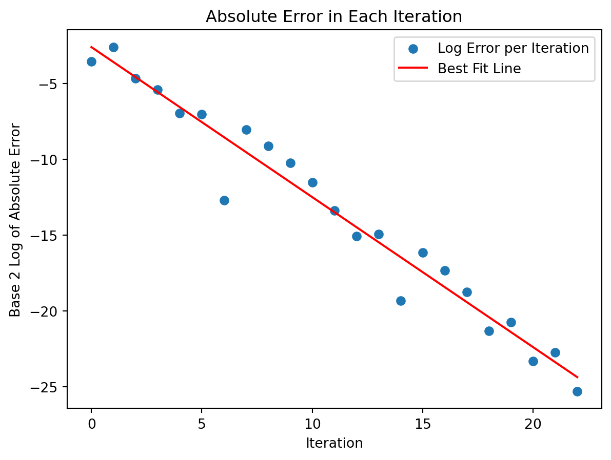
There will be times later in this course where we will not have a nice theorem like Theorem 4.2 and instead we will need to deduce the relationship from plots like these.
The trend is linear since logarithms and exponential functions are inverses. Hence, applying a logarithm to an exponential will give a linear function.
The slope of the resulting linear function should be \(-1\) in this case since we are dividing by a factor of 2 each iteration. Visually verify that the slope in the plot below follows this trend (the red dashed line in the plot is shown to help you see the slope).
Exercise 4.20 Carefully read and discuss all of the details of the previous example and plots. Then create plots similar to this example to solve a different equation to which you know the exact solution. You should see the same basic behaviour based on the theorem that you proved in Exercise 4.17. If you do not see the same basic behaviour then something has gone wrong.
Example 4.2 Another plot that numerical analysts use quite frequently for determining how an algorithm is behaving as it progresses is shown in Figure 4.5. and is defined by the following axes:
- The horizontal axis is the absolute error at iteration \(k\).
- The vertical axis is the absolute error at iteration \(k+1\).
def plot_error_progression(errors):
    # Calculating the log2 of the absolute error at step k and k+1
    log_errors = np.log2(errors)
    log_errors_k = log_errors[:-1]  # log errors at step k (excluding the last one)
    log_errors_k_plus_1 = log_errors[1:]  # log errors at step k+1 (excluding the first one)

    # Plotting log_errors_k+1 vs log_errors_k
    plt.scatter(log_errors_k, log_errors_k_plus_1, label='Log Error at k+1 vs Log Error at k')

    # Fitting a straight line to the data points
    slope, intercept = np.polyfit(log_errors_k, log_errors_k_plus_1, deg=1)
    best_fit_line = slope * log_errors_k + intercept
    plt.plot(log_errors_k, best_fit_line, color='red', label='Best Fit Line')

    # Setting up the plot
    plt.xlabel('Log2 of Absolute Error at Step k')
    plt.ylabel('Log2 of Absolute Error at Step k+1')
    plt.title('Log2 of Absolute Error at Step k+1 vs Step k')
    plt.legend()
    plt.show()

plot_error_progression(errors)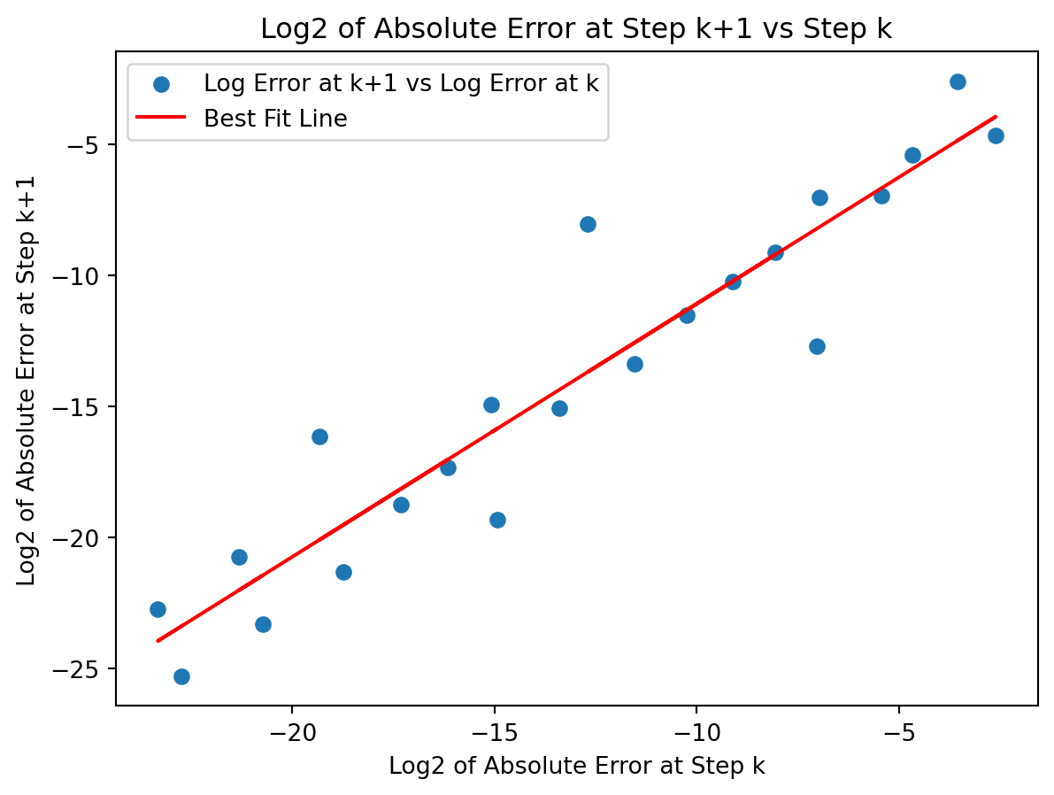
This type of plot takes a bit of explaining the first time you see it. Each point in the plot corresponds to an iteration of the algorithm. The x-coordinate of each point is the base-2 logarithm of the absolute error at step \(k\) and the y-coordinate is the base-2 logarithm of the absolute error at step \(k+1\). The initial interations are on the right-hand side of the plot where the error is the largest (this will be where the algorithm starts). As the iterations progress and the error decreases the points move to the left-hand side of the plot. Examining the slope of the trend line in this plot shows how we expect the error to progress from step to step. The slope appears to be about \(1\) in Figure 4.5 and the intercept appears to be about \(-1\). In this case we used a base-2 logarithm for each axis so we have just empirically shown that \[\begin{equation} \log_2(\text{absolute error at step $k+1$}) \approx 1\cdot \log_2(\text{absolute error at step $k$}) -1. \end{equation}\] Exponentiating both sides we see that this linear relationship turns into (You should stop now and do this algebra.) Rearranging a bit more we get \[\begin{equation} (\text{absolute error at step $k+1$}) = \frac{1}{2}(\text{absolute error at step $k$}), \end{equation}\] exactly as expected!! Pause and ponder this result for a second – we just empirically verified the convergence rate for the bisection method just by examining Figure 4.5. That’s what makes these types of plots so powerful!
Exercise 4.21 Reproduce plots like those in the previous example but for the different equation that you used in Exercise 4.20. Again check that the plots have the expected shape.
4.3 Fixed Point Iteration
We will now investigate a different problem that is closely related to root finding: the fixed point problem. Given a function \(g\) (of one real argument with real values), we look for a number \(p\) such that \[ g(p)=p. \] This \(p\) is called a fixed point of \(g\).
Any root finding problem \(f(x)=0\) can be reformulated as a fixed point problem, and this can be done in many (in fact, infinitely many) ways. For example, given \(f\), we can define \(g(x):=f(x) + x\); then \[ f(x) = 0 \quad \Leftrightarrow\quad g(x)=x. \] Just as well, we could set \(g(x):=\lambda f(x) + x\) with any \(\lambda\in{\mathbb R}\backslash\{0\}\), and there are many other possibilities.
The heuristic idea for approximating a fixed point of a function \(g\) is quite simple. We take an initial approximation \(x_{0}\) and calculate subsequent approximations using the formula \[ x_{n}:=g(x_{n-1}). \] A graphical representation of this sequence when \(g = \cos\) and \(x_0=2\) is shown in Figure 4.6.
To view the animation, click on the play button below the plot.
Exercise 4.22 The plot that emerges in Figure 4.6 is known as a cobweb diagram, for obvious reason. Explain to others in your group what is happening in the animation in Figure 4.6 and how that animation is related to the fixed point iteration \(x_{n} = \cos(x_{n-1})\).
Exercise 4.23 🎓 The animation in Figure 4.6 is a graphical representation of the fixed point iteration \(x_{n} = \cos(x_{n-1})\). Use Python to calculate the first 10 iterations of this sequence with \(x_0=0.2\). Use that to get an estimate of the solution to the equation \(\cos(x)-x=0\).
Why is the sequence \((x_n)\) expected to approximate a fixed point? Suppose for a moment that the sequence \((x_n)\) converges to some number \(p\), and that \(g\) is continuous. Then \[ p=\lim_{n\to\infty}x_{n}=\lim_{n\to\infty}g(x_{n-1})= g\left(\lim_{n\to\infty}x_{n-1}\right)=g(p). \tag{4.1}\] Thus, if the sequence converges, then it converges to a fixed point. However, this resolves the problem only partially. One would like to know:
Under what conditions does the sequence \((x_n)\) converge?
How fast is the convergence, i.e., can one obtain an estimate for the approximation error?
So there is much for you to investigate!
Exercise 4.24 Copy the two plots in Figure 4.7 to a piece of paper and draw the first few iterations of the fixed point iteration \(x_{n} = g(x_{n-1})\) on each of them. In the first plot start with \(x_0=0.2\) and in the second plot start with \(x_0=1.5\) and in the second plot start with \(x=0.9\) What do you observe about the convergence of the sequence in each case?
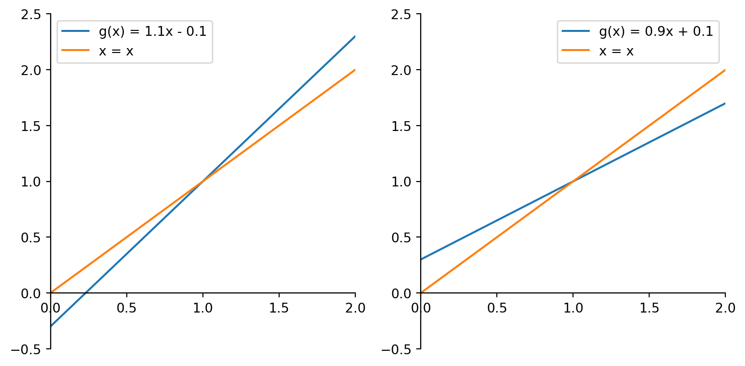
Can you make some conjectures about when the sequence \((x_n)\) will converge to a fixed point and when it will not?
Exercise 4.25 Make similar plots as in the previous exercise but with different slopes of the blue line. Can you make some conjectures about how the speed of convergence is related to the slope of the blue line?
Now see if your observations are in agreement with the following theorem:
Theorem 4.3 (Fixed Point Theorem) Suppose that \(g:[a,b]\to [a,b]\) is differentiable, and that there exists \(0<k<1\) such that \[ \lvert g^{\prime}(x)\rvert\leq k\quad \text{for all }x \in (a,b). \tag{4.2}\] Then, \(g\) has a unique fixed point \(p\in [a,b]\); and for any choice of \(x_0 \in [a,b]\), the sequence defined by \[ x_{n}:=g(x_{n-1}) \quad \text{for all }n\ge1 \tag{4.3}\] converges to \(p\). The following estimate holds: \[ \lvert p- x_{n}\rvert \leq k^n \lvert p-x_{0}\rvert \quad \text{for all }n\geq1. \tag{4.4}\]
Proof. The proof of this theorem is not difficult, but you can skip it and go directly to Exercise 4.26 if you feel that the theorem makes intuitive sense and you are not interested in proofs.
We first show that \(g\) has a fixed point \(p\) in \([a,b]\). If \(g(a)=a\) or \(g(b)=b\) then \(g\) has a fixed point at an endpoint. If not, then it must be true that \(g(a)>a\) and \(g(b)<b\). This means that the function \(h(x):=g(x)-x\) satisfies \[ \begin{aligned} h(a) &= g(a)-a>0, & h(b)&=g(b)-b<0 \end{aligned} \] and since \(h\) is continuous on \([a,b]\) the Intermediate Value Theorem guarantees the existence of \(p\in(a,b)\) for which \(h(p)=0\), equivalently \(g(p)=p\), so that \(p\) is a fixed point of \(g\).
To show that the fixed point is unique, suppose that \(q\neq p\) is a fixed point of \(g\) in \([a,b]\). The Mean Value Theorem implies the existence of a number \(\xi\in(\min\{p,q\},\max\{p,q\})\subseteq(a,b)\) such that \[ \frac{g(p)-g(q)}{p-q}=g'(\xi). \] Then \[ \lvert p - q\rvert = \lvert g(p)-g(q) \rvert = \lvert (p-q)g'(\xi) \rvert = \lvert p-q\rvert \lvert g'(\xi) \rvert \le k\lvert p-q\rvert < \lvert p-q\rvert, \] where the inequalities follow from Eq. 4.2. This is a contradiction, which must have come from the assumption \(p\neq q\). Thus \(p=q\) and the fixed point is unique.
Since \(g\) maps \([a,b]\) onto itself, the sequence \(\{x_n\}\) is well defined. For each \(n\ge0\) the Mean Value Theorem gives the existence of a \(\xi\in(\min\{x_n,p\},\max\{x_n,p\})\subseteq(a,b)\) such that \[ \frac{g(x_n)-g(p)}{x_n-p}=g'(\xi). \] Thus for each \(n\ge1\) by Eq. 4.2, Eq. 4.3 \[ \lvert x_n-p\rvert = \lvert g(x_{n-1})-g(p) \rvert = \lvert (x_{n-1}-p)g'(\xi) \rvert = \lvert x_{n-1}-p\rvert \lvert g'(\xi) \rvert \le k\lvert x_{n-1}-p\rvert. \] Applying this inequality inductively, we obtain the error estimate Eq. 4.4. Moreover since \(k <1\) we have \[\lim_{n\rightarrow\infty}\lvert x_{n}-p\rvert \le \lim_{n\rightarrow\infty} k^n \lvert x_{0}-p\rvert = 0, \] which implies that \((x_n)\) converges to \(p\). ◻
Exercise 4.26 🎓 This exercise shows why the conditions of the Theorem 4.3 are important.
The equation \[ f(x)=x^{2}-2=0 \] has a unique root \(\sqrt{2}\) in \([1, 2]\). There are many ways of writing this equation in the form \(x=g(x)\); we consider two of them: \[ \begin{aligned} x&=g(x)=x-(x^{2}-2), & x&=h(x)=x-\frac{x^{2}-2}{3}. \end{aligned} \] Calculate the first terms in the sequences generated by the fixed point iteration procedures \(x_{n}=g(x_{n-1})\) and \(x_{n}=h(x_{n-1})\) with start value \(x_0=1\). Which of these fixed point problems generate a rapidly converging sequence? Calculate the derivatives of \(g\) and \(h\) and check if the conditions of the fixed point theorem are satisfied.
The previous exercise illustrates that one needs to be careful in rewriting root finding problems as fixed point problems—there are many ways to do so, but not all lead to a good approximation. In the next section about Newton’s method we will discover a very good choice.
Note at this point that Theorem 4.3 gives only sufficient conditions for convergence; in practice, convergence might occur even if the conditions are violated.
Exercise 4.27 🎓 In this exercise you will write a Python function to implement the fixed point iteration algorithm.
For implementing the fixed point method as a computer algorithm, there’s one more complication to be taken into account: how many steps of the iteration should be taken, i.e., how large should \(n\) be chosen, in order to reach the desired precision? The error estimate in Eq. 4.4 is often difficult to use for this purpose because it involves estimates on the derivative of \(g\) which may not be known.
Instead, one uses a different stopping condition for the algorithm. Since the sequence is expected to converge rapidly, one uses the difference \(|x_n-x_{n-1}|\) to measure the precision reached. If this difference is below a specified limit, say \(\tau\), the iteration is stopped. Since it is possible that the iteration does not converge—see the example above—one would also stop the iteration (with an error message) if a certain number of steps is exceeded, in order to avoid infinite loops. In pseudocode the fixed point iteration algorithm is then implemented as follows:
Fixed point iteration
\[ \begin{array}{ll} \ 1: \ \textbf{function} \ FixedPoint(g,x_0,tol, N) &\sharp \ function \ g, \ start \ point \ x_0,\\ \ 2: \ \quad x \gets x_0; \ n \gets 0 &\sharp \ tolerance \ tol,\\ \ 3: \ \quad \textbf{for} \ i \gets 1 \ \textbf{to}\ N &\sharp \ max. \ num. \ of \ iterations \ N \\ \ 4: \ \quad\quad y \gets x; \ x \gets g(x) & \\ \ 5: \ \quad\quad \textbf{if} \ |y-x| < tol \ \textbf{then} &\sharp \ Desired \ tolerance \ reached \\ \ 6: \ \quad\quad\quad \textbf{return} \ x & \\ \ 7: \ \quad\quad \textbf{end \ if} & \\ \ 8: \ \quad \textbf{end for} & \\ \ 9: \ \quad \textbf{exception}(Iteration \ has \ not \ converged) & \\ 10: \ \textbf{end function} & \end{array} \] Implement this algorithm in Python. Use it to approximate the fixed point of the function \(g(x)=\cos(x)\) with start value \(x_0=2\) and tolerance \(tol=10^{-8}\).
Further reading: Section 2.2 of (Burden and Faires 2010).
4.4 Newton’s Method
In the Bisection Method (Section 4.2) we had used only the sign of of the function at the guessed points. We will now investigate how we can use also the value and the slope (derivative) of the function to get a much improved method.
4.4.1 Intuition
Root finding is really the process of finding the \(x\)-intercept of the function. If the function is complicated (e.g. highly nonlinear or does not lend itself to traditional by-hand techniques) then we can approximate the \(x\)-intercept by creating a Taylor Series approximation of the function at a nearby point and then finding the \(x\)-intercept of that simpler Taylor Series. The simplest non-trivial Taylor Series is a linear function – a tangent line!
Exercise 4.28 A tangent line approximation to a function \(f(x)\) near a point \(x_0\) is \[\begin{equation} y = f(x_0) + f'(x_0) \left( x - x_0 \right). \end{equation}\] Set \(y\) to zero and solve for \(x\) to find the \(x\)-intercept of the tangent line. \[\begin{equation} \text{$x$-intercept of tangent line is } x = \underline{\hspace{0.5in}} \end{equation}\]
The idea of approximating the function by its tangent line gives us an algorithm for approximating the root of a function:
Given a value of \(x\) that is a decent approximation of the root, draw a tangent line to \(f(x)\) at that point.
Find where the tangent line intersects the \(x\) axis.
Use this intersection as the new \(x\) value and repeat.
The first step has been shown for you in Figure 4.8. The tangent line to the function \(f(x)\) at the point \((x_0, f(x_0))\) is shown in red. The \(x\)-intercept of the tangent line is the new \(x\) value, \(x_1\). The process is then repeated with \(x_1\) as the new \(x_0\) and so on.
The graphical method illustrated in Figure 4.8 was introduced by Sir Isaac Newton and is therefore known as Newton’s Method. Joseph Raphson then gave the algebraic formulation and popularised the method, which is therefore also known as the Newton-Raphson method.
Exercise 4.29 If we had started not at \(x_0\) in Figure 4.8 but instead at the very end of the x-axis in that figure, what would have happened? Would this initial guess have worked to eventually approximate the root?
Exercise 4.30 Sketch some other function \(f(x)\) with a root and choose an initial point \(x_0\) and graphically perform the Newton iteration a few times, similar to Figure 4.8. Does the algorithm appear to converge to the root in your example? Do you think that this will generally take more or fewer steps than the Bisection Method?
Exercise 4.31 🎓 Consider the function \(f(x)=\sin(x)+1\). It has roots at \(x=2n\pi+3\pi/2\) for \(n\in\mathbb{Z}\). However at the roots we have \(f'(x)=0\). Make yourself a sketch to see why. What will happen when you apply Newton’s method with a starting value of \(x_0=\pi\)? You should be able to answer this just by looking at the sketch.
Exercise 4.32 Using your result from Exercise 4.28, write the formula for the \(x\)-intercept of the tangent line to \(f(x)\) at the point \((x_n, f(x_n))\). This is the formula for the next guess \(x_{n+1}\) in Newton’s Method. Newton’s method is a fixed point iteration method of the form \(x_{n+1} = g(x_{n})\) with \[ g(x)= \dots. \] Fill in the blank in the above formula.
Exercise 4.33 🎓 Apply Newton’s method to find the root of the function \(f(x) = x^2 - 2\) with an initial guess of \(x_0=1\). Calculate the first two iterations of the sequence by hand (you do not need a calculator or computer for this). Use a calculator or computer to calculate the next two iterations and fill in the following table:
| \(n\) | \(x_n\) | \(f(x_n)\) | \(f'(x_n)\) |
|---|---|---|---|
| \(0\) | \(x_0 = 1\) | \(f(x_0) = -1\) | \(f'(x_0) = 2\) |
| \(1\) | \(x_1 = 1 - \frac{-1}{2} = \frac{3}{2}\) | \(f(x_1) =\) | \(f'(x_1) =\) |
| \(2\) | \(x_2 =\) | \(f(x_2) =\) | \(f'(x_2) =\) |
| \(3\) | \(x_3 =\) | \(f(x_3) =\) | \(f'(x_3) =\) |
| \(4\) | \(x_4 =\) |
4.4.2 Implementation
Exercise 4.34 The following is an outline a Python function called newton() for Newton’s method. The function needs to accept a Python function for \(f(x)\), a Python function for \(f'(x)\), an initial guess, and an optional error tolerance.
def newton(f, fprime, x0, tol=1e-12):
    """
    Find root of f(x) using Newton's Method.

    Parameters:
        f (function): Function whose root we want to find
        fprime (function): Derivative of f
        x0 (float): Initial guess for the root
        tol (float, optional): Error tolerance. Defaults to 1e-6

    Returns:
        float: Approximate root of f(x)
        or error message if method fails
    """

    # Set x equal to initial guess x0

    # Loop for maximum of 30 iterations:
    #   1. Calculate next Newton iteration:
    #      x_new = x - f(x)/f'(x)

    #   2. Check if within tolerance:
    #      If |x_new - x| < tol, return x_new as root
    #      If not, update x = x_new

    # 3. If loop completes without finding root,
    #    return message that method did not converge
Exercise 4.35 🎓 Use your implementation from Exercise 4.34 to approximate the root of the function \(f(x) = x^2 - 2\) with an initial guess of \(x_0=1\). Use a tolerance of \(10^{-12}\).
4.4.3 Failures
There are several ways in which Newton’s Method will behave unexpectedly – or downright fail. Some of these issues can be foreseen by examining the Newton iteration formula \[\begin{equation} x_{n+1} = x_n - \frac{f(x_n)}{f'(x_n)}. \end{equation}\] Some of the failures that we will see are a little more surprising. Also in this section we will look at the convergence rate of Newton’s Method and we will show that we can greatly outperform the Bisection method.
Exercise 4.36 There are several reasons why Newton’s method could fail. Work with your partners to come up with a list of reasons. Support each of your reasons with a sketch or an example.
Exercise 4.37 One of the failures of Newton’s Method is that it requires a division by \(f'(x_n)\). If \(f'(x_n)\) is zero then the algorithm completely fails. Go back to your Python function and put an if statement in the function that catches instances when Newton’s Method fails in this way.
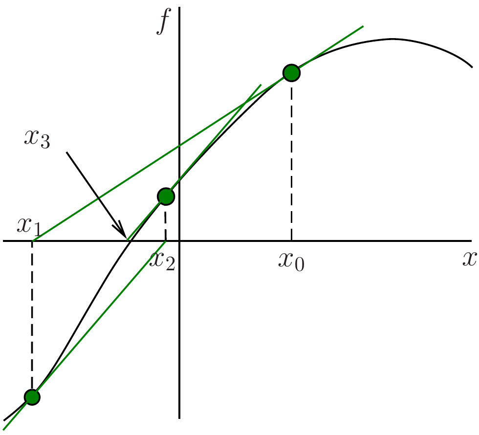
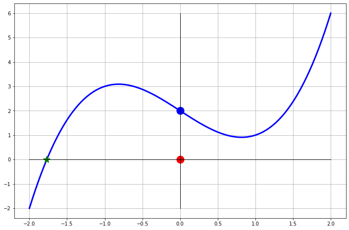
Exercise 4.38 An interesting failure can occur with Newton’s Method that you might not initially expect. Consider the function \(f(x) = x^3 - 2x + 2\). This function has a root near \(x=-1.77\). Fill in the table below by hand. You really do not need a computer for this. Then draw the tangent lines into Figure 4.9 for approximating the solution to \(f(x) = 0\) with a starting point of \(x=0\).
| \(n\) | \(x_n\) | \(f(x_n)\) | \(f'(x_n)\) |
|---|---|---|---|
| \(0\) | \(x_0 = 0\) | \(f(x_0) = 2\) | \(f'(x_0) = -2\) |
| \(1\) | \(x_1 = 0 - \frac{f(x_0)}{f'(x_0)} = 1\) | \(f(x_1) = 1\) | \(f'(x_1) = 1\) |
| \(2\) | \(x_2 = 1 - \frac{f(x_1)}{f'(x_1)} =\) | \(f(x_2) =\) | \(f'(x_2) =\) |
| \(3\) | \(x_3 =\) | \(f(x_3) =\) | \(f'(x_3) =\) |
| \(4\) | \(x_4 =\) | \(f(x_4) =\) | \(f'(x_4) =\) |
| \(\vdots\) | \(\vdots\) | \(\vdots\) | \(\vdots\) |
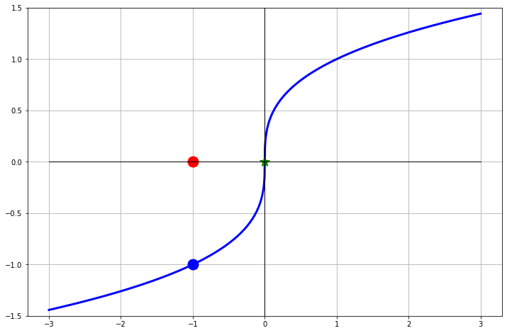
Exercise 4.39 Now let us consider the function \(f(x) = \sqrt[3]{x}\). This function has a root \(x=0\). Furthermore, it is differentiable everywhere except at \(x=0\) since \[\begin{equation} f'(x) = \frac{1}{3} x^{-2/3} = \frac{1}{3x^{2/3}}. \end{equation}\] The point of this exercise is to show what can happen when the point of non-differentiability is precisely the point that you are looking for.
- Fill in the table of iterations starting at \(x=-1\), draw the tangent lines on the plot, and make a general observation of what is happening with the Newton iterations.
| \(n\) | \(x_n\) | \(f(x_n)\) | \(f(x_n)\) |
|---|---|---|---|
| \(0\) | \(x_0 = -1\) | \(f(x_0) = -1\) | \(f'(x_0) =\) |
| \(1\) | \(x_1 = -1 - \frac{f(-1)}{f'(-1)} =\) | \(f(x_1) =\) | \(f'(x_1) =\) |
| \(2\) | |||
| \(3\) | |||
| \(4\) | |||
| \(\vdots\) | \(\vdots\) | \(\vdots\) | \(\vdots\) |
Now let us look at the Newton iteration in a bit more detail. Since \(f(x) = x^{1/3}\) and \(f'(x) = \frac{1}{3} x^{-2/3}\) the Newton iteration can be simplified as \[\begin{equation} x_{n+1} = x_n - \frac{x_n^{1/3}}{ \left( \frac{1}{3} x_n^{-2/3} \right)} = x_n - 3 \frac{x_n^{1/3}}{x_n^{-2/3}} = x_n - 3x_n = -2x_n. \end{equation}\] What does this tell us about the Newton iterations?
Hint: You should have found the exact same thing in the numerical experiment in part 1.Was there anything special about the starting point \(x_0=-1\)? Will this problem exist for every starting point?
Exercise 4.40 Repeat the previous exercise with the function \(f(x) = x^3 - 5x\) with the starting point \(x_0 = -1\).
4.4.4 Rate of Convergence
We saw in Example 4.2 how we could empirically determine the rate of convergence of the bisection method by plotting the error in the new iterate on the \(y\)-axis and the error in the old iterate on the \(x\) axis of a log-log plot. Take a look at that example again and make sure you understand the code and the explanation of the plot. Then, to investigate the rate of convergence of Newton’s method you can do the same thing.
Exercise 4.41 🎓 Write a Python function newton_with_error_tracking() that returns a list of absolute errors between the iterates and the exact solution. You can start with your code from newton() from Exercise 4.34 and add the collection of the errors in a list as in the bisection_with_error_tracking() function that we wrote in Example 4.1. Your new function should accept a Python function for \(f(x)\), a Python function for \(f'(x)\), the exact root, an initial guess, and an optional error tolerance.
Then, use this function to list the error progression for Newton’s method for finding the root of \(f(x) = x^2 - 2\) with the initial guess \(x_0 = 1\) and tolerance \(10^{-12}\). You should find that the error goes down extremely quickly and that for the final iteration Python can no longer detect a difference between the new iterate and its own value for \(\sqrt{2}\).
Exercise 4.42
Plot the errors you calculated in Exercise 4.41 using the
plot_error_progression()function that we wrote in Example 4.2. Note that you will first need to remove the zeros from the error list, otherwise you will get an error. You can remind yourself of how to work with lists in Section 1.3.2.Give a thorough explanation for how to interpret the plot that you just made.
🎓 Extract the slope and intercept of the line that you fitted to the log-log plot of the error progression using the
np.polyfitfunction. What does this tell you about how the error at each iteration is related to the error at the previous iteration?
Exercise 4.43 Reproduce plots like those in the previous example but for the different equation that you used in Exercise 4.20. Again check that the plots have the expected shape.
4.5 The Secant Method
4.5.1 Intuition and Implementation
Newton’s Method has second-order (quadratic) convergence and, as such, will perform faster than the Bisection method. However, Newton’s Method requires that you have a function and a derivative of that function. The conundrum here is that sometimes the derivative is cumbersome or impossible to obtain but you still want to have the great quadratic convergence exhibited by Newton’s method.
Recall that Newton’s method is \[\begin{equation} x_{n+1} = x_n - \frac{f(x_n)}{f'(x_n)}. \end{equation}\] If we replace \(f'(x_n)\) with an approximation of the derivative then we may have a method that is close to Newton’s method in terms of convergence rate but is less troublesome to compute. Any method that replaces the derivative in Newton’s method with an approximation is called a Quasi-Newton Method.
The first, and most obvious, way to approximate the derivative is just to use the slope of a secant line instead of the slope of the tangent line in the Newton iteration. If we choose two starting points that are quite close to each other then the slope of the secant line through those points will be approximately the same as the slope of the tangent line.
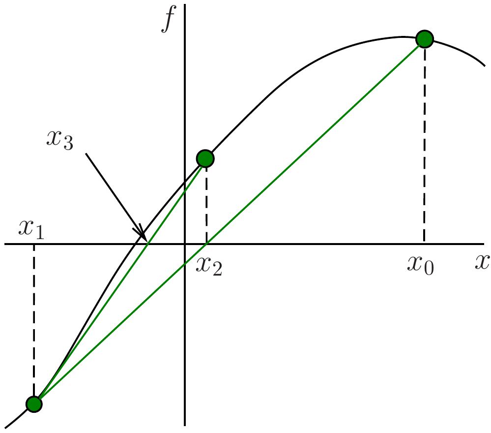
Exercise 4.44 Use the backward difference \[\begin{equation} f'(x_n) \approx \frac{f(x_n) - f(x_{n-1})}{x_n - x_{n-1}} \end{equation}\] to approximate the derivative of \(f\) at \(x_n\). Discuss why this approximates the derivative. Use this approximation of \(f'(x_n)\) in the expression for \(x_{n+1}\) of Newton’s method. Show that that the result simplifies to \[\begin{equation} x_{n+1} = x_n - \frac{f(x_n)\left( x_n - x_{n-1} \right)}{f(x_n) - f(x_{n-1})}. \end{equation}\]
Exercise 4.45 Notice that the iteration formula for \(x_{n+1}\) that you derived depends on both \(x_n\) and \(x_{n-1}\). So to start the iteration you need to choose two points \(x_0\) and \(x_1\) before you can calculate \(x_2, x_3, \dots\). Draw several pictures showing what the secant method does pictorially. Discuss whether it is important to choose these starting points close to the root and close to each other.
Exercise 4.46 🎓 Write a Python function for solving equations of the form \(f(x) = 0\) with the secant method. Your function should accept a Python function, two starting points, and an optional error tolerance. Also write a test script that clearly shows that your code is working.
4.5.2 Analysis
Up to this point we have done analysis work on the Bisection Method and Newton’s Method. We have found that the methods are first order and second order respectively. We end this chapter by doing the same for the Secant Method.
Exercise 4.47 Write a function secant_with_error_tracking() that returns a list of absolute errors between the iterates and the exact solution. You can start with your code from secant() from Exercise 4.46 and add the collection of the errors in a list as in the bisection_with_error_tracking() function that we wrote in Example 4.1. Your new function should accept a Python function, the exact root, two starting points, and an optional error tolerance.
Use this function to list the error progression for the secant method for finding the root of \(f(x) = x^2 - 2\) with the starting points \(x_0 = 1\) and \(x_1 = 3\). Use a tolerance of \(10^{-12}\). Use the plot_error_progression() function that we wrote in Example 4.2 to plot the error progression.
Exercise 4.48 🎓 Using the np.polyfit function, extract the slope of the line that you had fit to the log-log plot of the error progression in Exercise 4.47. What does this slope tell you about how the error at each iteration is related to the error at the previous iteration?
Exercise 4.49 Make error progression plots for a few different functions and look at the slopes. What do you notice?
4.6 Order of Convergence
You will by now have noticed that Newton’s method converges much faster than the bisection method. The secant method also converges faster than the bisection method, though not quite as fast as Newton’s method. You will have observed that reflected in the different slopes of the error progression graphs. In this section we summarize your observations theoretically. Thus this section is untypical in that it does not contain further explorations for you to do but instead just consolidates what you have already done. In class this will be presented as a lecture.
4.6.1 Definition
Definition 4.1 Suppose that \(x_{n}\to p\) as \(n\to\infty\) and \(x_n\neq p\) for all \(n\). The sequence \(\{x_{n}\}\) is said to have order of convergence \(\alpha \ge 1\) if there exists a constant \(\lambda >0\) such that \[ \lim_{n\to\infty}\frac{E_{n+1}}{E_{n}^{\alpha}}=\lambda . \tag{4.5}\] Here \(E_n\) denotes the absolute error in the \(n\)th approximation: \(E_{n}=\vert x_{n}-p\vert\).
If \(\alpha=1,2,3,\dots\), the convergence is said to be linear, quadratic, cubic, \(\dots\), respectively. Note that if the convergence is linear, then the positive constant \(\lambda\) that appears in the above definition must be smaller than 1 (\(0<\lambda<1\)), because otherwise the sequence will not converge.
A sequence with a higher order of convergence converges much more rapidly than a sequence with a lower order of convergence. To see this, let us consider the following example:
Example 4.3 Let \(\{x_{n}\}\) and \(\{y_{n}\}\) be sequences converging to zero and let, for \(n\geq 0\), \[ \vert x_{n+1}\vert = k \vert x_{n}\vert \quad \text{ and } \quad \vert y_{n+1}\vert = k \vert y_{n}\vert^{2}, \tag{4.6}\] where \(0< k < 1\). According to the definition, \(\{x_{n}\}\) is linearly convergent and \(\{y_{n}\}\) is quadratically convergent.
Also, we have \[ \begin{split} \vert x_{n}\vert&=k\vert x_{n-1}\vert= k^{2}\vert x_{n-2}\vert=...=k^{n}\vert x_{0}\vert ,\\ \vert y_{n}\vert&=k\vert y_{n-1}\vert^{2}= k\vert k\vert y_{n-2}\vert^{2}\vert^{2}=k^{3}\vert y_{n-2}\vert^{4}= k^{7}\vert y_{n-3}\vert^{8}=... =k^{2^{n}-1}\vert y_{0}\vert^{2^{n}}. \end{split} \tag{4.7}\] This illustrates that the quadratic convergence is much faster that the linear convergence.
We have defined the order of convergence of a converging sequence. We will also say than an iterative method has order of convergence \(\alpha\) if the sequence of approximations that it produces on a generic problem has order of convergence \(\alpha\).
4.6.2 Fixed Point Iteration
Suppose that \(g(x)\) satisfies the conditions of the Fixed Point Theorem on interval \([a,b]\), so that the sequence \(\{x_{n}\}\) generated by the formula \(x_{n+1}=g(x_{n})\) with \(x_{0}\in [a,b]\) converges to a fixed point \(p\). Then, using the Mean Value Theorem, we obtain \[ \begin{split} E_{n+1}&=\vert x_{n+1}-p\vert=\vert g(x_{n})-g(p)\vert\\ &=\vert g'(\xi_n)( x_{n}-p)\vert = E_{n}\vert g'(\xi_{n})\vert, \end{split} \tag{4.8}\] where \(\xi_{n}\) is a number between \(x_n\) and \(p\). This implies that if \(x_n\to p\), then \(\xi_n\to p\) as \(n\to\infty\). Therefore, \[ \lim_{n\to\infty}\frac{E_{n+1}}{E_{n}}=\vert g'(p)\vert . \tag{4.9}\] In general, \(g'(p)\neq 0\), so that the fixed point iteration produces a linearly convergent sequence.
Can the fixed-point iteration produce convergent sequences with convergence of order 2, 3, etc. ? It turns out that, under certain conditions, this is possible.
We will prove the following
Theorem 4.4 Let \(m > 1\) be an integer, and let \(g\in C^{m}[a,b]\). Suppose that \(p\in [a,b]\) is a fixed point of \(g\), and a point \(x_{0}\in [a,b]\) exists such that the sequence generated by the formula \(x_{n+1}=g(x_{n})\) converges to \(p\). If \(g'(p)=\dots =g^{(m-1)}(p)=0\), then \(\{x_{n}\}\) has the order of convergence \(m\).
Proof. Expanding \(g(x_{n})\) in Taylor’s series at point \(p\), we obtain: \[ \begin{split} x_{n+1}=g(x_{n}) &= g(p) + (x_{n}-p)g'(p)+\dots \\ &\qquad + \frac{(x_{n}-p)^{m -1}}{(m -1)!}g^{(m -1)}(p)\\ &\qquad + \frac{(x_{n}-p)^{m}}{m!}g^{(m)}(\xi_n) \\ &=p+\frac{(x_{n}-p)^{m}}{(m)!}g^{(m)}(\xi_n), \end{split} \tag{4.10}\] where \(\xi_n\) is between \(x_{n}\) and \(p\) and, therefore, in \([a,b]\) (\(x_{n}\in[a,b]\) at least for sufficiently large \(n\)). Then we have \[ \begin{split} E_{n+1}&=\vert x_{n+1}-p\vert=\vert g(x_{n})-p\vert= \left\vert\frac{(x_{n}-p)^{m}}{(m)!}g^{(m)}(\xi_n)\right\vert\\ &= E_{n}^m \frac{\vert g^{(m)}(\xi_n)\vert}{m!}. \end{split} \tag{4.11}\] Therefore (using the fact that \(\xi_n\to p\)), \[ \lim_{n\to\infty}\frac{E_{n+1}}{E_{n}^m}= \frac{\vert g^{(m)}(p)\vert}{m!} , \tag{4.12}\] which means that \(\{x_{n}\}\) has convergence of order \(m\).
4.6.3 Newton’s Method
Newton’s method for approximating the root \(p\) of the equation \(f(x)=0\) is equivalent to the fixed-point iteration \(x_{n+1}=g(x_{n})\) with \[ g(x)=x-\frac{f(x)}{f'(x)}. \tag{4.13}\] Suppose that sequence \(\{x_{n}\}\) converges to \(p\) and \(f'(p)\neq 0\). We have \[ g'(x)=\frac{f(x)f''(x)}{[f'(x)]^2} \quad \Rightarrow \quad g'(p)=\frac{f(p)f''(p)}{[f'(p)]^2}=0 . \tag{4.14}\] It follows from the above theorem that the order of convergence of Newton’s method is 2 (except in the special case where \(g''(p)=0\)).
4.6.4 Secant Method
The situation with the secant method is more complicated (since it cannot be reduced to the fixed point iteration) and requires a separate treatment. The result is that the secant method has order of convergence \(\alpha=\frac{1+\sqrt{5}}{2}\approx 1.618\).
Note that \(\alpha\) is known as the golden ratio. If you are intrigued to see the golden ratio appear in this context, you can find a proof below. If you are happy to just accept the miracle, you can skip the proof and go on to Section 4.7.
Suppose that a sequence \(\{x_{n}\}\), generated by the secant method \[ x_{n+1}=x_{n}- \frac{f(x_{n})(x_{n}-x_{n-1})}{f(x_{n})-f(x_{n-1})}, \tag{4.15}\] converges to \(p\). Let \[ e_{n}=x_{n}-p, \tag{4.16}\] so that \(E_n=\vert e_n\vert\), and we assume that \(E_n \ll 1\), which is definitely true for sufficiently large \(n\) (since the sequence \(\{x_n\}\) is converging to \(p\)). Subtracting \(p\) from both sides of Eq. 4.15, we obtain \[ e_{n+1}=e_{n}- \frac{f(p+e_{n})(e_{n}-e_{n-1})}{f(p+e_{n})-f(p+e_{n-1})}, \tag{4.17}\] Expanding \(f(p+e_{n})\) and \(f(p+e_{n-1})\) in Taylor series about \(p\) and taking into account that \(f(p)=0\), we find that \[ \begin{split} f(p+e_{n})&=e_{n}f^{\prime}(p)+ \frac{e_{n}^{2}}{2}f^{\prime\prime}(p)+ \cdots \\ &=e_{n}f^{\prime}(p)(1+e_{n}Q)+ \cdots,\\ f(p+e_{n-1})&=e_{n-1}f^{\prime}(p)+ \frac{e_{n-1}^{2}}{2}f^{\prime\prime}(p)+ \cdots \\ &=e_{n-1}f^{\prime}(p)(1+e_{n-1}Q)+ \cdots, \end{split} \tag{4.18}\] where \[ Q=\frac{f^{\prime\prime}(p)}{2f^{\prime}(p)}. \tag{4.19}\] Substitution of Eq. 4.18 into Eq. 4.17 yields \[ \begin{split} e_{n+1}&=e_{n}- \frac{e_{n}(e_{n}-e_{n-1})f^{\prime}(p)(1+e_{n}Q)+\cdots}{f^{\prime}(p) \left[e_{n}-e_{n-1}+Q(e_{n}^2-e_{n-1}^2)+\cdots\right]} \\ &=e_{n}\left(1-\frac{1+e_{n}Q+\cdots}{1+Q(e_{n}+e_{n-1})+\cdots}\right). \end{split} \tag{4.20}\] Since, for small \(x\), \[ \frac{1}{1+x+\cdots}= 1-x+\cdots , \tag{4.21}\] we obtain \[ \begin{split} e_{n+1}&=e_{n}\left(1-\left(1+e_{n}Q+\cdots\right)\left(1-Q(e_{n}+e_{n-1})+\cdots\right)\right)\\ &=Q e_{n}e_{n-1}+\cdots. \end{split} \tag{4.22}\] Thus, for sufficiently large \(n\), we have \[ e_{n+1} \approx Q e_{n}e_{n-1}. \tag{4.23}\] Hence, \[ E_{n+1} \approx \vert Q\vert \, E_{n}E_{n-1}. \tag{4.24}\] Now we assume that (for all sufficiently large \(n\)) \[ E_{n+1} \approx \lambda E_{n}^{\alpha}, \tag{4.25}\] where \(\lambda\) and \(\alpha\) are positive constants. Substituting Eq. 4.25 into Eq. 4.24, we find \[ \lambda E_{n}^{\alpha} \approx \vert Q\vert E_{n}E_{n-1} \quad \text{ or } \quad \lambda E_{n}^{\alpha-1} \approx \vert Q\vert E_{n-1}. \tag{4.26}\] Applying Eq. 4.25 one more time (with \(n\) replaced by \(n-1\)), we obtain \[ \lambda \left(\lambda E_{n-1}^{\alpha}\right)^{\alpha-1} \approx \vert Q\vert E_{n-1} \tag{4.27}\] or, equivalently, \[ \lambda^{\alpha} E_{n-1}^{\alpha(\alpha-1)} \approx \vert Q\vert E_{n-1}. \tag{4.28}\] The last equation will be satisfied provided that \[ \lambda^{\alpha}=\vert Q\vert, \quad \alpha(\alpha-1)=1 , \tag{4.29}\] which requires that \[ \lambda=\vert Q\vert^{1/\alpha}, \quad \alpha=(1+\sqrt{5})/2\approx 1.62. \tag{4.30}\] Thus, we have shown that if \(\{x_{n}\}\) is a convergent sequence generated by the secant method, then \[ \lim_{n\to\infty}\frac{E_{n+1}}{E_{n}^{\alpha}}=\vert Q\vert^{1/\alpha}. \tag{4.31}\] Thus, the secant method has superlinear convergence.
Further reading: Section 2.4 of (Burden and Faires 2010).
4.7 Algorithm Summaries
The following four problems are meant to have you re-build each of the algorithms that we developed in this chapter. Write all of the mathematical details completely and clearly. Do not just write “how” the method works, but give all of the mathematical details for “why” it works.
Exercise 4.50 Let \(f(x)\) be a continuous function on the interval \([a,b]\) where \(f(a) \cdot f(b) < 0\). Clearly give all of the mathematical details for how the Bisection Method approximates the root of the function \(f(x)\) in the interval \([a,b]\).
Exercise 4.51 Let \(f(x)\) be a differentiable function with a root near \(x=x_0\). Clearly give all of the mathematical details for how Newton’s Method approximates the root of the function \(f(x)\).
Exercise 4.52 Let \(f(x)\) be a continuous function with a root near \(x=x_0\). Clearly give all of the mathematical details for how the Secant Method approximates the root of the function \(f(x)\).
4.8 Problems
Exercise 4.53 Can the Bisection Method or Newton’s Method be used to find the roots of the function \(f(x) = \cos(x) + 1\)? Explain why or why not for each technique? What is the rate of convergence? Be careful here, the answer is surprising.
Exercise 4.54 How many iterations of the bisection method are necessary to approximate \(\sqrt{3}\) to within \(10^{-3}\), \(10^{-4}\), …, \(10^{-15}\) using the initial interval \([a,b]=[0,2]\)? See Theorem 4.2.
Exercise 4.55 Refer back to Example 4.1 and demonstrate that you get the same results for the order of convergence when solving the problem \(x^3 - 3 = 0\). Generate versions of all of the plots from that example and give thorough descriptions of what you learn from each plot.
Exercise 4.56 In this problem you will demonstrate that all of your root finding codes work. At the beginning of this chapter we proposed the equation solving problem \[\begin{equation} 3\sin(x) + 9 = x^2 - \cos(x). \end{equation}\] Write a script that calls upon your Bisection, Newton, and Secant methods one at a time to find the positive solution to this equation. Your script needs to output the solutions in a clear and readable way so you can tell which answer came from which root finding algorithm.
Exercise 4.57 In Figure 4.13 you see six different log-log plots of the new error to the old error for different root finding techniques. What is the order of the approximate convergence rate for each of these methods?
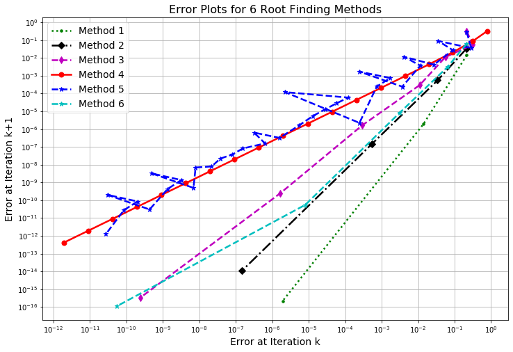
- In your own words, what does it mean for a root finding method to have a “first order convergence rate?” “Second order convergence rate?” etc.
Exercise 4.58 There are MANY other root finding techniques beyond the four that we have studied thus far. We can build these methods using Taylor Series as follows:
Near \(x=x_0\) the function \(f(x)\) is approximated by the Taylor Series \[\begin{equation} f(x) \approx y = f(x_0) + \sum_{n=1}^N \frac{f^{(n)}(x_0)}{n!} (x-x_0)^n \end{equation}\] where \(N\) is a positive integer. In a root-finding algorithm we set \(y\) to zero to find the root of the approximation function. The root of this function should be close to the actual root that we are looking for. Therefore, to find the next iterate we solve the equation \[\begin{equation} 0 = f(x_0) + \sum_{n=1}^N \frac{f^{(n)}(x_0)}{n!} (x-x_0)^n \end{equation}\] for \(x\). For example, if \(N=1\) then we need to solve \(0 = f(x_0) + f'(x_0)(x-x_0)\) for \(x\). In doing so we get \(x = x_0 - f(x_0)/f'(x_0)\). This is exactly Newton’s method. If \(N=2\) then we need to solve \[\begin{equation} 0 = f(x_0) + f'(x_0)(x-x_0) + \frac{f''(x_0)}{2!}(x-x_0)^2 \end{equation}\] for \(x\).
Solve for \(x\) in the case that \(N=2\). Then write a Python function that implements this root-finding method.
Demonstrate that your code from part (a) is indeed working by solving several problems where you know the exact solution.
Show several plots that estimates the order of the method from part (a). That is, create a log-log plot of the successive errors for several different equation-solving problems.
What are the pro’s and con’s to using this new method?
Exercise 4.59 (modified from (Burden and Faires 2010)) An object falling vertically through the air is subject to friction due to air resistance as well as gravity. The function describing the position of such an object is \[\begin{equation} s(t) = s_0 - \frac{mg}{k} t + \frac{m^2 g}{k^2}\left( 1- e^{-kt/m} \right), \end{equation}\] where \(m\) is the mass measured in kg, \(g\) is gravity measured in meters per second per second, \(s_0\) is the initial position measured in meters, and \(k\) is the coefficient of air resistance.
What are the dimensions of the parameter \(k\)?
If \(m = 1\)kg, \(g=9.8\)m/s\(^2\), \(k=0.1kg/s\), and \(s_0 = 100\)m how long will it take for the object to hit the ground? Find your answer to within 0.01 seconds.
The value of \(k\) depends on the aerodynamics of the object and might be challenging to measure. We want to perform a sensitivity analysis on your answer to part (b) subject to small measurement errors in \(k\). If the value of \(k\) is only known to within 10% then what are your estimates of when the object will hit the ground?
Exercise 4.60 In Single Variable Calculus you studied methods for finding local and global extrema of functions. You likely recall that part of the process is to set the first derivative to zero and to solve for the independent variable (remind yourself why you are doing this). The trouble with this process is that it may be very very challenging to solve by hand. This is a perfect place for Newton’s method or any other root finding technique!
Find the local extrema for the function \(f(x) = x^3(x-3)(x-6)^4\) using numerical techniques where appropriate.
Exercise 4.61 (scipy.optimize.fsolve()) The scipy library in Python has many built-in numerical analysis routines much like the ones that we have built in this chapter. Of particular interest to the task of root finding is the fsolve command in the scipy.optimize library.
Go to the help documentation for
scipy.optimize.fsolveand make yourself familiar with how to use the tool.First solve the equation \(x\sin(x) - \log(x) = 0\) for \(x\) starting at \(x_0 = 3\).
Make a plot of the function on the domain \([0,5]\) so you can eyeball the root before using the tool.
Use the
scipy.optimize.fsolve()command to approximate the root.Fully explain each of the outputs from the
scipy.optimize.fsolve()command. You should use thefsolve()command withfull_output=1so you can see all of the solver diagnostics.
Demonstrate how to use
fsolve()using any non-trivial nonlinear equation solving problem. Demonstrate what some of the options offsolve()do.The
scipy.optimize.fsolve()command can also solve systems of equations (something we have not built algorithms for in this chapter). Consider the system of equations \[\begin{equation} \begin{aligned} x_0 \cos(x_1) &= 4 \\ x_0 x_1 - x_1 &= 5 \end{aligned} \end{equation}\] The following Python code allows you to usescipy.optimize.fsolve()so solve this system of nonlinear equations in much the same way as we did in part (b) of this problem. However, be aware that we need to think ofxas a vector of \(x\)-values. Go through the code below and be sure that you understand every line of code.
import numpy as np
from scipy.optimize import fsolve

def F(x):
 return [x[0]*np.cos(x[1])-4, x[0]*x[1] - x[1] - 5]

fsolve(F, [6,1], full_output=1)
# Note: full_output=1 gives the solver diagnostics- Solve the system of nonlinear equations below using
.fsolve(). \[\begin{equation} \begin{aligned} x^2-xy^2 &=2 \\ xy &= 2 \end{aligned} \end{equation}\]
4.9 Projects
At the end of every chapter we propose a few projects related to the content in the preceding chapter(s). In this section we propose two ideas for a project related to numerical algebra. The projects in this book are meant to be open ended, to encourage creative mathematics, to push your coding skills, and to require you to write and communicate your mathematics.
4.9.1 Basins of Attraction
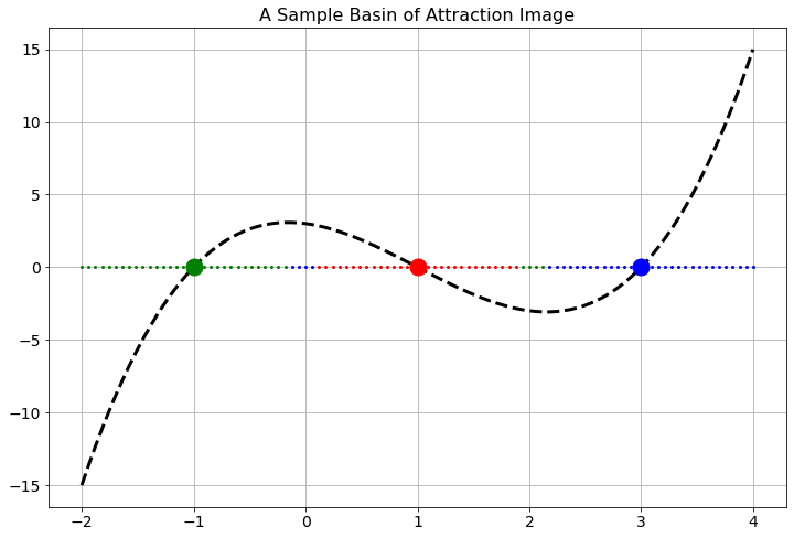
Let \(f(x)\) be a differentiable function with several roots. Given a starting \(x\) value we should be able to apply Newton’s Method to that starting point and we will converge to one of the roots (so long as you are not in one of the special cases discussed earlier in the chapter). It stands to reason that starting points near each other should all end up at the same root, and for some functions this is true. However, it is not true in general.
A basin of attraction for a root is the set of \(x\) values that converges to that root under Newton iterations. In this problem you will produce coloured plots showing the basins of attraction for all of the following functions. Do this as follows:
Find the actual roots of the function by hand (this should be easy on the functions below).
Assign each of the roots a different colour.
Pick a starting point on the \(x\) axis and use it to start Newton’s Method.
Colour the starting point according to the root that it converges to.
Repeat this process for many many starting points so you get a coloured picture of the \(x\) axis showing where the starting points converge to.
The set of points that are all the same colour are called the basin of attraction for the root associated with that colour. In Figure 4.14 there is an image of a sample basin of attraction image.
Create a basin on attraction image for the function \(f(x) = (x-4)(x+1)\).
Create a basin on attraction image for the function \(g(x) = (x-1)(x+3)\).
Create a basin on attraction image for the function \(h(x) = (x-4)(x-1)(x+3)\).
Find a non-trivial single-variable function of your own that has an interesting picture of the basins of attraction. In your write up explain why you thought that this was an interesting function in terms of the basins of attraction.
Now for the fun part! Consider the function \(f(z) = z^3 - 1\) where \(z\) is a complex variable. That is, \(z = x + iy\) where \(i = \sqrt{-1}\). From the Fundamental Theorem of Algebra we know that there are three roots to this polynomial in the complex plane. In fact, we know that the roots are \(z_0 = 1\), \(z_1 = \frac{1}{2}\left( -1 + \sqrt{3} i \right)\), and \(z_2 = \frac{1}{2} \left( -1 - \sqrt{3} i \right)\) (you should stop now and check that these three numbers are indeed roots of the polynomial \(f(z)\)). Your job is to build a picture of the basins of attraction for the three roots in the complex plane. This picture will naturally be two-dimensional since numbers in the complex plane are two dimensional (each has a real and an imaginary part). When you have your picture give a thorough write up of what you found.
Now pick your favourite complex-valued function and build a picture of the basins of attraction. Consider this an art project! See if you can come up with the prettiest basin of attraction picture.
4.9.2 Artillery
An artillery officer wishes to fire his cannon on an enemy brigade. He wants to know the angle to aim the cannon in order to strike the target. If we have control over the initial velocity of the cannon ball, \(v_0\), and the angle of the cannon above horizontal, \(\theta\), then the initial vertical component of the velocity of the ball is \(v_y(0) = v_0 \sin(\theta)\) and the initial horizontal component of the velocity of the ball is \(v_x(0) = v_0 \cos(\theta)\). In this problem we will assume the following:
We will neglect air resistance1 so, for all time, the differential equations \(v_y'(t) = -g\) and \(v_x'(t) = 0\) must both hold.
We will assume that the position of the cannon is the origin of a coordinate system so \(s_x(0) = 0\) and \(s_y(0) = 0\).
We will assume that the target is at position \((x_*,y_*)\) which you can measure accurately relative to the cannon’s position. The landscape is relatively flat but \(y_*\) could be a bit higher or a bit lower than the cannon’s position.
Use the given information to write a nonlinear equation2 that relates \(x_*\), \(y_*\), \(v_0\), \(g\), and \(\theta\). We know that \(g = 9.8m/s^2\) is constant and we will assume that the initial velocity can be adjusted between \(v_0 = 100m/s\) and \(v_0 = 150m/s\) in increments of \(10m/s\). If we then are given a fixed value of \(x_*\) and \(y_*\) the only variable left to find in your equation is \(\theta\). A numerical root-finding technique can then be applied to your equation to approximate the angle. Create several look up tables for the artillery officer so they can be given \(v_0\), \(x_*\), and \(y_*\) and then use your tables to look up the angle at which to set the cannon. Be sure to indicate when a target is out of range.
Write a brief technical report detailing your methods. Support your work with appropriate mathematics and plots. Include your tables at the end of your report.
Burden, Richard L., and J. Douglas Faires. 2010. Numerical Analysis. 9th ed. Brooks Cole.
Strictly speaking, neglecting air resistance is a poor assumption since a cannon ball moves fast enough that friction with the air plays a non-negligible role. However, the assumption of no air resistance greatly simplifies the maths and makes this version of the problem more tractable. The second version of the artillery problem in Chapter 8 will look at the effects of air resistance on the cannon ball.↩︎
Hint: Symbolically work out the amount of time that it takes until the vertical position of the cannon ball reaches \(y_*\). Then substitute that time into the horizontal position, and set the horizontal position equation to \(x_*\)↩︎