6 Integrals
Now that we understand how to calculate derivatives, we begin our work on the second principal computation of calculus: evaluating a definite integral. You will be able to transfer much of what you did in the previous chapter, where you investigated the errors in numerical differentiation, to the investigation of the errors in numerical integration.
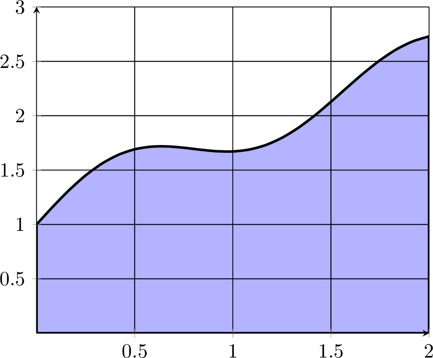
Exercise 6.1 Remember that a single-variable definite integral can be interpreted as the signed area between the curve and the \(x\) axis. Consider the shaded area of the region under the function plotted in Figure 6.1 between \(x=0\) and \(x=2\).
What rectangle with area 6 gives an upper bound for the area under the curve? Can you give a better upper bound?
Why must the area under the curve be greater than 3?
Is the area greater than 4? Why/Why not?
Work with your group to give an estimate of the area and provide an estimate for the amount of error that you are making.
In this chapter we will study three different techniques for approximating the value of a definite integral.
6.1 Riemann Sums
In this subsection we will build our first method for approximating definite integrals. Recall from Calculus that the definition of the Riemann integral is \[\begin{equation} \int_a^b f(x) dx = \lim_{\Delta x \to 0} \sum_{j=1}^N f(x_j) \Delta x, \end{equation}\] where \(N\) is the number of sub intervals on the interval \([a,b]\) and \(\Delta x\) is the width of the interval. As with differentiation, we can remove the limit and have a decent approximation of the integral so long as \(N\) is large (or equivalently, as long as \(\Delta x\) is small). \[\begin{equation} \int_a^b f(x) dx \approx \sum_{j=1}^N f(x_j) \Delta x. \end{equation}\] You are likely familiar with this approximation of the integral from Calculus. The value of \(x_j\) can be chosen anywhere within the sub interval and three common choices are to use the left-aligned, the midpoint-aligned, and the right-aligned.
We see a depiction of this in Figure 6.2.
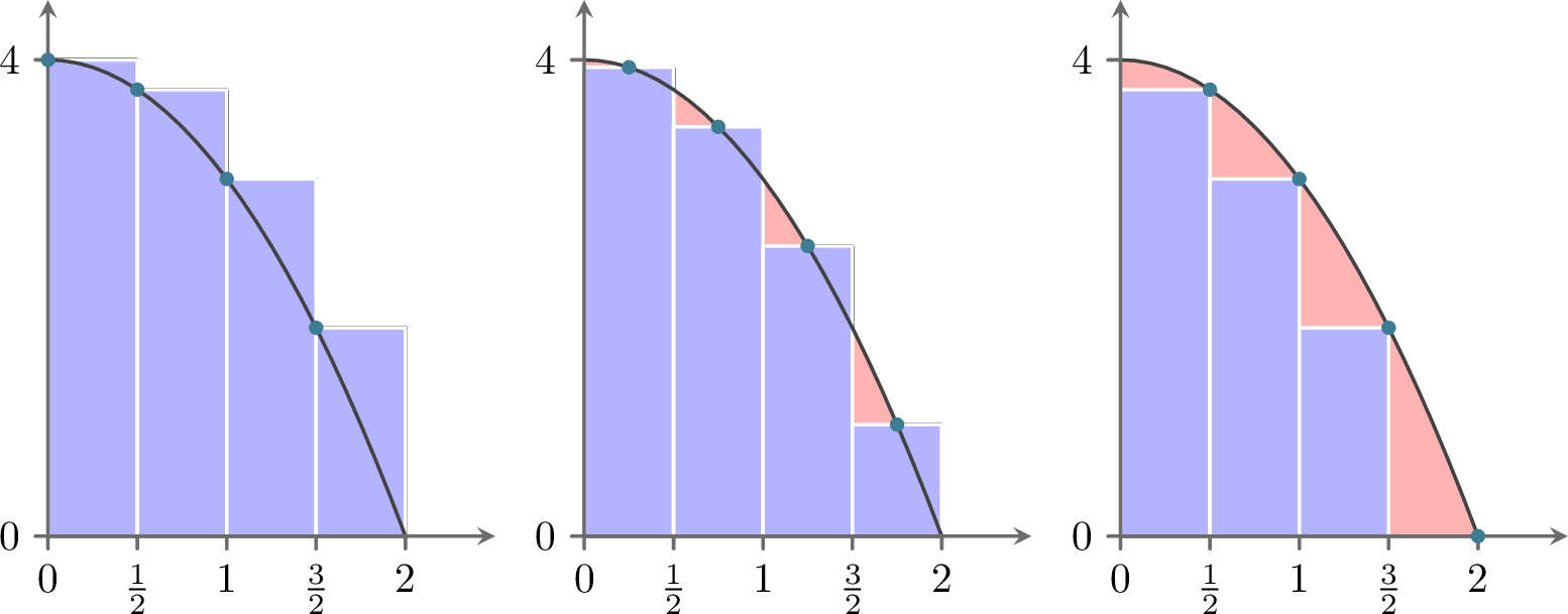
Clearly, the more rectangles we choose the closer the sum of the areas of the rectangles will get to the integral.
Exercise 6.2 🎓 Write a Python function RiemannSum(f, a, b, N, method='left') that approximates an integral with a Riemann sum. Your Python function should accept a Python Function f, a lower bound a, an upper bound b, the number of subintervals N, and an optional input method that allows the user to designate whether they want ‘left’, ‘right’, or ‘midpoint’ rectangles. Test your code on several functions for which you know the integral. You should write your code without any loops.
Exercise 6.3 Consider the function \(f(x) = \sin(x)\). We know the antiderivative for this function, \(F(x) = -\cos(x) + C\). In this question we are going to get a sense of the order of the error when doing Riemann Sum integration.
Find the exact value of \[\begin{equation} I=\int_0^{1} f(x) dx. \end{equation}\]
Now calculate left Riemann Sum approximation (using your
RiemannSum()function from Exercise 6.2) with various values of \(\Delta x\). Fill in the table with your results. Note the similarity between this exercise and Exercise 5.8 where you created a similar table for approximating a derivative. If you want to save yourself tedious work, you may want to adapt the code from Exercise 5.9 to this exercise.
| \(\Delta x\) | Approx. Integral | Absolute Error |
|---|---|---|
| \(2^{-1} = 0.5\) | ||
| \(2^{-2} = 0.25\) | ||
| \(2^{-3}\) | ||
| \(2^{-4}\) | ||
| \(2^{-5}\) | ||
| \(2^{-6}\) | ||
| \(2^{-7}\) | ||
| \(2^{-8}\) |
- There was nothing really special about powers of 2 in part (2) of this exercise. Examine other sequences of \(\Delta x\) with a goal toward answering the question:
If we find an approximation of the integral with a fixed \(\Delta x\) and find an absolute error, then what would happen to the absolute error if we divide \(\Delta x\) by some positive constant \(M\)?
Exercise 6.4 Repeat the previous exercise using the midpoint Riemann sum. Again answer the question what happens to the absolute error if we divide \(\Delta x\) by some positive constant \(M\).
Exercise 6.5 Create a plot with the width of the subintervals on the horizontal axis and the absolute error between your Riemann sum calculations (left, right, and midpoint) and the exact integral for a known definite integral of your choice. Your plot should be on a log-log scale. Based on your plot, what is the approximate order of the error in the Riemann sum approximation? Again notice the similarity between this exercise and Exercise 5.17 where you created a similar plot for approximating a derivative. And don’t be worried if you plot three lines but can only see two of them. The third line is likely very close to one of the other two.
6.2 Trapezoidal Rule
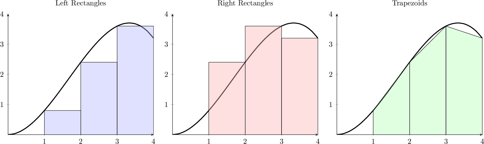
Now let us turn our attention to some slightly better algorithms for calculating the value of a definite integral: The Trapezoidal Rule and Simpson’s Rule. There are many others, but in practice these two are relatively easy to implement and have reasonably good error approximations. To motivate the idea of the trapezoidal rule consider Figure 6.3. It is plain to see that trapezoids will make better approximations than rectangles at least in this particular case. Another way to think about using trapezoids, however, is to see the top side of the trapezoid as a secant line connecting two points on the curve. As \(\Delta x\) gets arbitrarily small, the secant lines become better and better approximations for tangent lines and are hence arbitrarily good approximations for the curve. For these reasons it seems like we should investigate how to systematically approximate definite integrals via trapezoids.
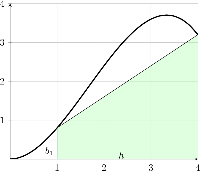
Exercise 6.6 Consider a single trapezoid approximating the area under a curve. From geometry we recall that the area of a trapezoid is \[\begin{equation} A = \frac{1}{2}\left( b_1 + b_2 \right) h, \end{equation}\] where \(b_1, b_2\) and \(h\) are marked in Figure 6.4. The function shown in the picture is \(f(x) = \frac{1}{5} x^2 (5-x)\). Find the area of the shaded region as an approximation to \[\begin{equation} \int_1^4 \left( \frac{1}{5} x^2 (5-x) \right) dx. \end{equation}\]
Now use the same idea with \(h = \Delta x = 1\) to approximate the area under the function using three trapezoids, as illustrated in the last panel of Figure 6.3.
Exercise 6.7 (Trapezoidal Rule) Now generalise the idea from Exercise 6.6 to divide the interval \([a,b]\) into \(N\) subintervals with boundaries \(\{x_0=a, x_1, x_2, \ldots, x_{N-1},x_N=b\}\). Fill in the missing bits in the equations below. The area of the trapezoid on the subinterval from \(x_{j-1}\) to \(x_j\) is \[\begin{equation} A_j = \frac{1}{2} \left[ f(???) + f(???) \right]\left(??? - ??? \right). \end{equation}\] Then the approximation of the integral is \[\begin{equation} \int_a^b f(x) dx \approx \sum_{???}^{???} A_j. \end{equation}\]
Exercise 6.8 🎓 Write a Python function Trapezoidal(f, a, b, N) that approximates an integral with the trapezoidal method you derived in the previous exercise. Your Python function should accept a Python Function f, a lower bound a, an upper bound b and the number of subintervals N. You should write your code without any loops. Test your code on several functions for which you know the integral.
Exercise 6.9 You have by now developed and repeatedly used ways to investigate how the errors for numerical integration and differentiation schemes depend on the stepsize. It is now up to you to do the same for the trapezoidal rule. Remember that the goal is to answer the question:
If I approximate the integral with a fixed \(\Delta x\) and find an absolute error of \(P\), then what will the absolute error be using a width of \(\Delta x / M\)?
You can either do this with a table or with a graph. What is the order of the error for the trapezoidal rule?
6.3 Simpsons Rule
The trapezoidal rule does a decent job approximating integrals, but ultimately you are using linear functions to approximate \(f(x)\) and the accuracy may suffer if the step size is too large or the function too non-linear. You likely notice that the trapezoidal rule will give an exact answer if you were to integrate a linear or constant function. A potentially better approach would be to get an integral that evaluates quadratic functions exactly. We call this method Simpson’s Rule after Thomas Simpson (1710-1761) who, by the way, was a basket weaver in his day job so he could pay the bills and keep doing math.
Three points are needed to uniquely determine a quadratic function, where two points were enough to uniquely determine a linear function. So for Simpson’s method we need to evaluate the function at three points (not two as for the trapezoidal rule). To approximate the integral a function \(f(x)\) on the interval \([a,b]\) we will use the three points \((a,f(a))\), \((m,f(m))\), and \((b,f(b))\) where \(m=\frac{a+b}{2}\) is the midpoint of the two boundary points.
We want to find constants \(A_1\), \(A_2\), and \(A_3\) in terms of \(a\), \(b\), \(f(a)\), \(f(b)\), and \(f(m)\) such that \[\begin{equation} \int_a^b f(x) dx = A_1 f(a) + A_2 f(m) + A_3 f(b) \end{equation}\] is exact for all constant, linear, and quadratic functions. This would guarantee that we have an exact integration method for all polynomials of order 2 or less but should serve as a decent approximation if the function is not quadratic.
Exercise 6.10 Follow these steps to find \(A_1\), \(A_2\), and \(A_3\).
Verify that \[\begin{equation} \int_a^b 1 dx = b-a = A_1 + A_2 + A_3. \end{equation}\]
Verify that \[\begin{equation} \int_a^b x dx = \frac{b^2 - a^2}{2} = A_1 a + A_2 \left( \frac{a+b}{2} \right) + A_3 b. \end{equation}\]
Verify that \[\begin{equation} \int_a^b x^2 dx = \frac{b^3 - a^3}{3} = A_1 a^2 + A_2 \left( \frac{a+b}{2} \right)^2 + A_3 b^2. \end{equation}\]
Verify that the above linear system of equations has the solution \[\begin{equation} A_1 = \frac{b-a}{6}, \quad A_2 = \frac{4(b-a)}{6}, \quad \text{and} \quad A_3 = \frac{b-a}{6}. \end{equation}\]
Exercise 6.11 At this point we can see that an integral can be approximated as \[\begin{equation} \int_a^b f(x) dx \approx \left( \frac{b-a}{6} \right) \left( f(a) + 4f\left( \frac{a+b}{2} \right) + f(b) \right) \end{equation}\] and the technique will give an exact answer for any polynomial of order 2 or below.
Verify the previous sentence by integrating \(f(x) = 1\), \(f(x) = x\) and \(f(x) = x^2\) by hand on the interval \([0,1]\) and using the approximation formula.
To make the punchline of the previous exercises a bit more clear: Using the formula \[\begin{equation} \int_a^b f(x) dx \approx \left( \frac{b-a}{6} \right) \left( f(a) + 4 f(m) + f(b) \right) \end{equation}\] is the same as fitting a parabola to the three points \((a,f(a))\), \((m,f(m))\), and \((b,f(b))\) and finding the area under the parabola exactly. That is exactly the step up from the trapezoidal rule and Riemann sums that we were after:
Riemann sums approximate the function with constant functions,
the trapezoidal rule uses linear functions, and
now we have a method for approximating with parabolas.
To improve upon this idea we now examine the problem of partitioning the interval \([a,b]\) into small pieces and running this process on each piece. This is called Simpson’s Rule for integration.
Exercise 6.12 (Simpson’s Rule) We divide the interval \([a,b]\) into \(N\) subintervals with boundaries \(\{x_0=a, x_1, x_2, \ldots, x_{N-1},x_N=b\}\). Fill in the missing bits in the equations below. We approximate the integral on the subinterval from \(x_{j-1}\) to \(x_j\) by \[\begin{equation} A_j = \frac{1}{???} \left[ f(???) + ??? f(???)+f(???) \right]\left(??? - ??? \right). \end{equation}\] Then the approximation of the integral is \[\begin{equation} \int_a^b f(x) dx \approx \sum_{???}^{???} A_j. \end{equation}\]
Exercise 6.13 🎓 Write a Python function Simpsons(f, a, b, N) that approximates an integral with Simpson’s rule that you derived in the previous exercise. Your Python function should accept a Python Function f, a lower bound a, an upper bound b and the number of subintervals N. You should write your code without any loops. Test your code on several functions for which you know the integral.
Exercise 6.14 🎓 As in Exercise 6.9, use your favourite method to determine how the absolute error in Simpson’s rule depends on the step size and hence determine the order of the error for Simpson’s rule?
Exercise 6.15 Use the integration problem and exact answer \[\begin{equation} \int_0^{\pi/4} e^{3x} \sin(2x) dx = \frac{3}{13} e^{3\pi/4} + \frac{2}{13} \end{equation}\] and produce a log-log error plot with \(\Delta x\) on the horizontal axis and the absolute error on the vertical axis. Include one graph for each of our integration methods. Fully explain how the error rates show themselves in your plot.
Thus far we have three numerical approximations for definite integrals: Riemann sums (with rectangles), the trapezoidal rule, and Simpsons’s rule. There are MANY other approximations for integrals and we leave the further research to the curious reader.
Further reading: Sections 4.3 to 4.9 of (Burden and Faires 2010).
6.4 Algorithm Summaries
Exercise 6.16 Explain how to approximate the value of a definite integral with Riemann sums. When will the Riemann sum approximation be exact? Distinguish between left, right and midpoint Riemann sums. State how the error of these approximations depends on the step size, i.e., give the order of the error for each of the three Riemann sums.
Exercise 6.17 Explain how to approximate the value of a definite integral with the trapezoidal rule. When will the trapezoidal rule approximation be exact? What is the order of the Trapezoidal rule?
Exercise 6.18 Explain how to approximate the value of a definite integral with Simpson’s rule. Give the full mathematical details for where Simpson’s rule comes from. When will the Simpson’s rule approximation be exact? What is the order of Simpson’s rule?
6.5 Problems
Exercise 6.19 Numerically integrate each of the functions over the interval \([-1,2]\) with an appropriate technique and verify mathematically that your numerical integral is correct to 10 decimal places. Then provide a plot of the function along with its numerical first derivative.
\(f(x) = \frac{x}{1+x^4}\)
\(g(x) = (x-1)^3 (x-2)^2\)
\(h(x) = \sin\left(x^2\right)\)
Exercise 6.20 Write a function that implements the trapezoidal rule on a list of \((x,y)\) order pairs representing the integrand function. The list of ordered pairs should be read from a spreadsheet file. Create a test spreadsheet file and a test script showing that your function is finding the correct integral.
Exercise 6.21 Use numerical integration to answer the question in each of the following scenarios
- We measure the rate at which water is flowing out of a reservoir (in gallons per second) several times over the course of one hour. Estimate the total amount of water which left the reservoir during that hour.
| time (min) | 0 | 7 | 19 | 25 | 38 | 47 | 55 |
|---|---|---|---|---|---|---|---|
| flow rate (gal/sec) | 316 | 309 | 296 | 298 | 305 | 314 | 322 |
You can download the data directly from the github repository for this course with the code below.
import numpy as np
import pandas as pd
data = np.array(pd.read_csv('https://github.com/gustavdelius/NumericalAnalysis2025/raw/main/data/Calculus/waterflow.csv'))- The department of transportation finds that the rate at which cars cross a bridge can be approximated by the function \[\begin{equation} f(t) = \frac{22.8 }{3.5 + 7(t-1.25)^4} , \end{equation}\] where \(t=0\) at 4pm, and is measured in hours, and \(f(t)\) is measured in cars per minute. Estimate the total number of cars that cross the bridge between 4 and 6pm. Make sure that your estimate has an error less than 5% and provide sufficient mathematical evidence of your error estimate.
Exercise 6.22 Consider the integrals \[\begin{equation}
\int_{-2}^2 e^{-x^2/2} dx \quad \text{and} \quad \int_0^1 \cos(x^2) dx.
\end{equation}\] Neither of these integrals have closed-form solutions so a numerical method is necessary. Create a log-log plot that shows the errors for the integrals with different values of \(h\) (log of \(h\) on the \(x\)-axis and log of the absolute error on the \(y\)-axis). Write a complete interpretation of the log-log plot. To get the exact answer for these plots use Python’s scipy.integrate.quad command. (What we are really doing here is comparing our algorithms to Python’s scipy.integrate.quad() algorithm).
6.6 Projects
In this section we propose several ideas for projects related to numerical Calculus. These projects are meant to be open ended, to encourage creative mathematics, to push your coding skills, and to require you to write and communicate your mathematics.
6.6.1 Higher Order Integration
Riemann sums can be used to approximate integrals and they do so by using piecewise constant functions to approximate the function. The trapezoidal rule uses piece wise linear functions to approximate the function and then the area of a trapezoid to approximate the area. We saw earlier that Simpson’s rule uses piece wise parabolas to approximate the function. The process which we used to build Simpson’s rule can be extended to any higher-order polynomial. Your job in this project is to build integration algorithms that use piece wise cubic functions, quartic functions, etc. For each you need to show all of the mathematics necessary to derive the algorithm, provide several test cases to show that the algorithm works, and produce a numerical experiment that shows the order of accuracy of the algorithm.
6.6.2 Dam Integration
Go to the USGS water data repository:
https://maps.waterdata.usgs.gov/mapper/index.html.
Here you will find a map with information about water resources around the country.
Zoom in to a dam of your choice (make sure that it is a dam).
Click on the map tag then click “Access Data”
From the drop down menu at the top select either “Daily Data” or “Current / Historical Data.” If these options do not appear then choose a different dam.
Change the dates so you have the past year’s worth of information.
Select “Tab-separated” under “Output format” and press Go. Be sure that the data you got has a flow rate (ft\(^3\)/sec).
At this point you should have access to the entire data set. Copy it into a
csvfile and save it to your computer.
For the data that you just downloaded you have three tasks: (1) plot the data in a reasonable way giving appropriate units, (2) find the total amount of water that has been discharged from the dam during the past calendar year, and (3) report any margin of error in your calculation based on the numerical method that you used in part (2).
6.6.3 WHO Data Integration
Go to data.gov or the World Health Organization Data Repository and find a data set where the variables naturally lead to a meaningful definite integral. Use appropriate code to evaluate the definite integral. If your data appears to be subject to significant noise then you might want to smooth the data first before doing the integral. Write a few sentences explaining what the integral means in the context of the data. Be very cautious of the units on the data sets and the units of your answer.