10 Initial Value Problems
10.1 Introduction
The topic of this and the next chapter is to find approximate solutions to ordinary differential equations.
Let us briefly recall what an ordinary differential equation (ODE) is. A rather arbitrarily chosen example for an ODE (here, of second order) is \[ y''(x) + 4 y'(x) + \sqrt[3]{y(x)} + \cos(x) = 0. \tag{10.1}\] Equations like this are normally satisfied by many functions \(y(x)\): the problem has many solutions. In order to specify a uniquely solvable problem, one needs to fix initial values, i.e., the value of \(y\) and its first derivative at some point, say, at \(x=0\): \[ y''(x) + 4 y'(x) + \sqrt[3]{y(x)} + \cos(x) = 0, \quad y(0)=1,\; y'(0)=-2. \tag{10.2}\] This is a so-called initial-value problem (IVP). Another variant is to specify the value of \(y(x)\), but not of its derivative, at two different points: \[ y''(x) + 4 y'(x) + \sqrt[3]{y(x)} + \cos(x) = 0, \quad y(0)=2,\; y(1)=1. \tag{10.3}\] This is called a boundary value problem (BVP).
Both IVPs and BVPs have a unique solution (under certain mathematical conditions). However, while one can show on abstract grounds that these solutions exist, it is often not practicable to find an explicit expression for them. The best one can hope for is to approximate the solution numerically. This is exactly our topic: to find approximation algorithms for the solutions of IVPs (this chapter) and BVPs (in Chapter 11).
10.2 Euler’s Method
For studying initial value problems (IVPs) for ordinary differential equations, let us start with the simplest known approximation scheme: Euler’s method. We will focus on direct computations here, and defer more in-depth discussions of the mathematical foundations to later.
We consider an IVP for a first-order equation, of the form \[ y'(x) = f(x,y(x)), \quad a \leq x \leq b, \quad y(a) = \alpha. \tag{10.4}\] Here \(a\), \(b\) and \(\alpha\) are some real numbers, and \(f\) is a function \(\mathbb{R}^2 \to \mathbb{R}\). (For a concrete example, see Example 10.1 below.) Under certain conditions on \(f\) — to be discussed in Section 10.3 — one knows that the problem has a unique solution; that is, that there is exactly one function \(y(x)\) defined on \([a,b]\) which satisfies Eq. 10.4. We often call \(y(x)\) the exact solution of the IVP. However, it is often difficult or even impossible to find an explicit expression for \(y(x)\). Our aim here is to approximate the solution numerically.
10.2.1 The method
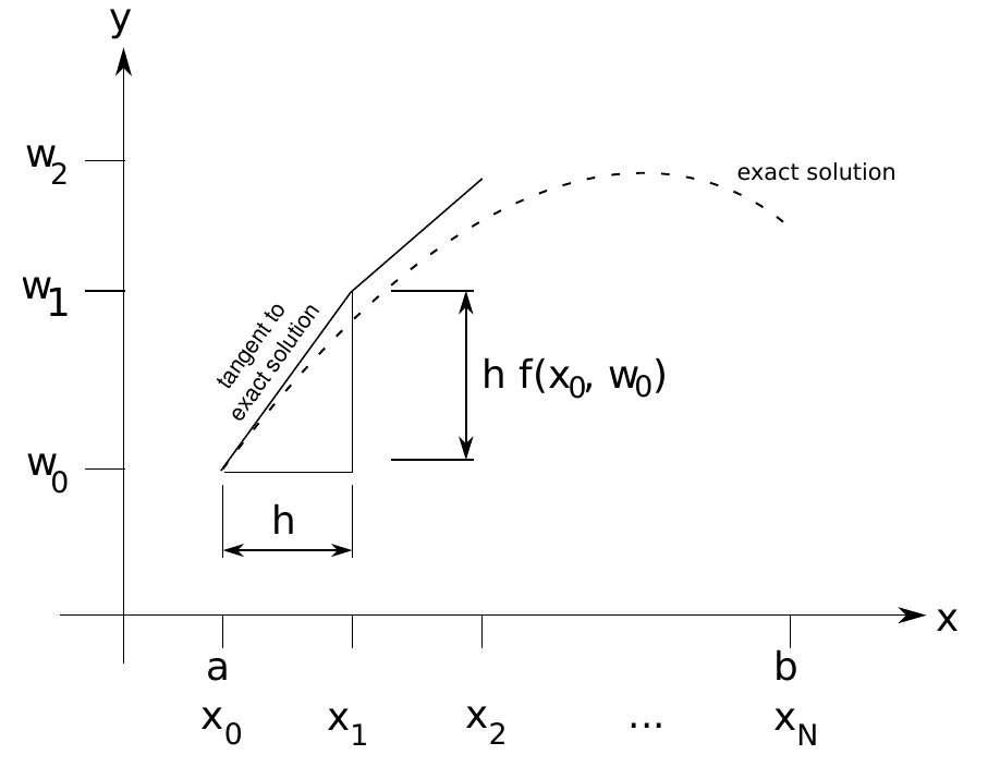
The idea behind Euler’s method is as follows (see Figure 10.1 for a visualization): We pick \(N \in \mathbb{N}\), and divide the interval \([a,b]\) into \(N\) subintervals of equal length, \(h = (b-a)/N\). The end points of these intervals are \[ x_i = a + i h, \quad i = 0,\ldots,N. \tag{10.5}\]
Terminology: \(N\) is called the number of steps and \(h\) is called the step size. The points \(x_0,\ldots,x_N\in[a,b]\) are referred to as mesh points.
We will approximate the exact solution \(y\) only at the mesh points \(x_i\); that is, we are looking for numbers \(w_0,\ldots,w_N\) such that \(y(x_i) \approx w_i\).
The first approximation \(w_0\) is easy to choose: We know that \(y\) satisfies the initial condition, \(y(x_0) = y(a) = \alpha\). Thus we set \(w_0:=\alpha\); this is even exact.
For finding \(w_1 \approx y(x_1)\), we use linear approximation: \[ \begin{split} y(x_1) &= y(x_0+h) \approx y(x_0) + h y'(x_0) \\ &\overset{(*)}{=} y(x_0) + h f(x_0,y(x_0)) = w_0 + hf(x_0,w_0). \end{split} \tag{10.6}\] For the equality \((*)\), we have used that \(y\) satisfies the ODE Eq. 10.4.
In the same way, we can find an approximation for \(y(x_2)\): \[ \begin{split} y(x_2) &= y(x_1+h) \approx y(x_1) + h y'(x_1) \\ &\overset{(*)}{=} y(x_1) + h f(x_1,y(x_1)) \overset{(\circ)}{\approx} w_1 + hf(x_1,w_1). \end{split} \tag{10.7}\] Our approximation value is \(w_2 := w_1 + hf(x_1,w_1)\). Note that we have used another approximation step \((\circ)\), using that \(y(x_1)\approx w_1\) and that \(f\) is sufficiently smooth; we will come back to this point in Section 10.2.2. We can continue the scheme for \(w_3\), \(w_4\), etc.: \[ w_0 := \alpha, \tag{10.8}\] \[ w_1 := w_0 + h f(x_0,w_0), \tag{10.9}\] \[ w_2 := w_1 + h f(x_1,w_1), \tag{10.10}\] \[\begin{equation*} \vdots \end{equation*}\] \[ w_{i+1} := w_i + h f(x_i,w_i). \tag{10.11}\] So the \(w_i\) are defined recursively. Eq. 10.11 is called the difference equation of Euler’s method.
Example 10.1 Let us consider the IVP \[ y'(x) = y(x)-x^2+1, \quad 0 \leq x \leq 1, \quad y(0) = \frac{1}{2}. \tag{10.12}\] In this case, the exact solution can be found using an integrating factor. It is
\[ y(x) = (x+1)^2-\frac{1}{2} e^x. \tag{10.13}\] This will allow us to compare the approximation with the exact solution. It is generally a good idea to test one’s numerical method on an example where one already knows the exact solution.
We choose \(N=10\) steps, i.e., \(h=1/10\). Here we shall only compute the first two steps. By Eq. 10.8, we certainly have \[ x_0 = 0, \quad w_0=\frac{1}{2}. \tag{10.14}\] This allows us to compute the approximation \(w_1\) at the mesh point \(x_1=1/10\), namely, by Eq. 10.9, \[ \begin{split} w_1&=w_0+h f(x_0,w_0) = w_0 + h (w_0-x_0^2+1)\\ &= \frac{1}{2} + \frac{1}{10} \left(\frac{1}{2}-0+1\right) = \frac{1}{2} + \frac{3}{20}\\ &= \frac{13}{20}. \end{split} \tag{10.15}\] Continuing the iteration to \(x_2=2/10\), we have by Eq. 10.10 that \[ \begin{split} w_2&=w_1+h f(x_1,w_1) = w_1 + h (w_1-x_1^2+1) \\ &= \frac{13}{20} + \frac{1}{10} \left(\frac{13}{20}-\left(\frac{1}{10}\right)^2+1 \right) = \frac{13}{20} + \frac{1}{10} \cdot \frac{174}{100}\\ &= \frac{407}{500}. \end{split} \tag{10.16}\]
Continuing further, we would obtain the values shown in Table 10.1. The values of the exact solution Eq. 10.13, evaluated to 9 decimals, are added for comparison. The last column, the error bound, will be discussed shortly.
| \(i\) | \(x_i\) | \(w_i\) | \(y(x_i)\) | \(|y(x_i)-w_i|\) | error bound |
|---|---|---|---|---|---|
| 0 | 0 | 0.5 | 0.5 | 0 | 0 |
| 1 | 0.1 | 0.65 | 0.657414541 | 0.007414541 | 0.0078878189 |
| 2 | 0.2 | 0.814 | 0.829298621 | 0.015298621 | 0.0166052069 |
| 3 | 0.3 | 0.9914 | 1.015070596 | 0.023670596 | 0.0262394106 |
| 4 | 0.4 | 1.18154 | 1.214087651 | 0.032547651 | 0.0368868524 |
| 5 | 0.5 | 1.383694 | 1.425639364 | 0.041945364 | 0.0486540953 |
| 6 | 0.6 | 1.5970634 | 1.648940600 | 0.051877200 | 0.0616589100 |
| 7 | 0.7 | 1.82076974 | 1.883123646 | 0.062353906 | 0.0760314530 |
| 8 | 0.8 | 2.053846714 | 2.127229536 | 0.073382822 | 0.0919155696 |
| 9 | 0.9 | 2.295231385 | 2.380198444 | 0.084967059 | 0.1094702333 |
| 10 | 1.0 | 2.543754524 | 2.640859086 | 0.097104562 | 0.1288711371 |
10.2.2 Error bounds
Denote the error at step \(i\) of Euler’s method by \[ \varepsilon_i=y(x_i)-w_i. \tag{10.17}\] Clearly \(\varepsilon_0=0\). We can represent \(\varepsilon_1\) as follows: assuming the second derivative \(y''\) exists on \((a,b)\), we can use Taylor’s Theorem to give \[ y(x_1)=y(x_0+h)=y(x_0)+hy'(x_0)+\frac{h^2y''(\xi_1)}{2} \tag{10.18}\] for some \(\xi_1\in(x_0,x_1)\). Now, \(y\) is a solution to the IVP so \(y(x_0)=y(a)=\alpha=w_0\) and \(y'(x_0)=f(x_0,y(x_0))=f(x_0,\alpha)=f(x_0,w_0)\) and, by definition of \(w_1\), \[ y(x_0)+hy'(x_0)=w_0+hf(x_0,w_0)=w_1. \tag{10.19}\] Substituting this gives \[ y(x_1)=w_1+\frac{h^2y''(\xi_1)}{2}. \tag{10.20}\] So the error after one step can be written as \[ \varepsilon_1=y(x_1)-w_1=\frac{h^2y''(\xi_1)}{2}. \tag{10.21}\] Although we do not know what \(y''(\xi_1)\) is, this does show how the error depends on the step length: it behaves like a multiple of \(h^2\).
We can now make an optimistic guess: if every step contributes a multiple of \(h^2\), then the total error at the end, after \(N\) steps, will be some multiple of \(Nh^2=(Nh)h=(b-a)h\). As \(h\to 0\), this tends to zero (whatever the unknown constants are) so the approximate solution converges to the exact solution. It turns out that this is basically correct, although much more careful reasoning is needed, as we shall see when we look at the error after the second step.
We can try to analyse the second step in the same way as the first step: use Taylor’s Theorem to write \[ y(x_2)=y(x_1+h)=y(x_1)+hy'(x_1)+\frac{h^2y''(\xi_2)}{2} \tag{10.22}\] and use the fact that \(y\) is a solution of the DE to substitute \(y'(x_1)=f(x_1,y(x_1))\): \[ y(x_2)=y(x_1)+hf(x_1,y(x_1))+\frac{h^2y''(\xi_2)}{2}. \tag{10.23}\] At this point, things look different: in the first step, we had \(y(x_0)=y(a)=\alpha\), but here we do not have \(y(x_1)=w_1\): the first step starts at \((x_0,w_0)=(a,\alpha)\), which lies exactly on the solution curve, but the second step starts at \((x_1,w_1)\), which does not lie on the solution curve. However, \(w_1\) is an approximation to \(y(x_1)\), and we have an expression for the error, namely \(\varepsilon_1\). Substituting \(y(x_1)=w_1+\varepsilon_1\) gives \[ y(x_2)=w_1+\varepsilon_1+hf(x_1,w_1+\varepsilon_1)+\frac{h^2y''(\xi_2)}{2}. \tag{10.24}\] Now, \(w_1+hf(x_1,w_1+\varepsilon_1)\) is very similar to the formula for \(w_2\): the only difference is that it has \(w_1+\varepsilon_1\), instead of \(w_1\). As we did for for \(y(x_1)\), we can think of this as being an approximation plus an error: \[ \underbrace{f(x_1,w_1+\varepsilon_1)}_{\text{exact}}=\underbrace{f(x_1,w_1)}_{\text{approx}}+ \underbrace{[f(x_1,w_1+\varepsilon_1)-f(x_1,w_1)]}_{\text{error}} \tag{10.25}\] leading to \[ y(x_2)=\varepsilon_1+\underbrace{w_1+hf(x_1,w_1)}_{=w_2}+h[f(x_1,w_1+\varepsilon_1)-f(x_1,w_1)]\frac{h^2y''(\xi_2)}{2}, \tag{10.26}\] which, as intended, forces \(w_2\) to appear: \[ y(x_2)=\varepsilon_1+w_2+h[f(x_1,w_1+\varepsilon_1)-f(x_1,w_1)]+\frac{h^2y''(\xi_2)}{2}. \tag{10.27}\] Subtracting \(w_2\) from both sides gives \[ \varepsilon_2=\varepsilon_1+h[f(x_1,w_1+\varepsilon_1)-f(x_1,w_1)]+\frac{h^2y''(\xi_2)}{2}. \tag{10.28}\] This describes the error at step 2 as the sum of three terms which can be thought of as:
\(\varepsilon_1\), the error carried forward from step 1;
\(h[f(x_1,w_1+\varepsilon_1)-f(x_1,w_1)]\), the error caused by starting at \((x_1,w_1)\), which is not on the solution curve;
\(h^2y''(\xi_2)/2\), the error built into Euler’s method by the approximation \(y(x+h)\approx y(x)+hy'(x)\).
This analysis works for every step: we have \[ \varepsilon_{i+1}=\varepsilon_i+h[f(x_i,w_i+\varepsilon_i)-f(x_i,w_i)]+\frac{h^2y''(\xi_{i+1})}{2}, \tag{10.29}\] where \(\xi_{i+1}\in(x_i,x_{i+1})\). This is a recurrence relation for \(\varepsilon_i\), and \(\varepsilon_0=0\). Now, we need to ask how large the different contributions can be. For the truncation error inherent in Euler’s method, we simply assume that there is a constant \(M\) such that \(|y''(x)|\leq M\) for all \(x\in[a,b]\). For the error associated with starting away from the solution curve, we use Taylor’s Theorem yet again: assuming \(f\) is differentiable in the second variable, we can write \[ f(x_i,w_i+\varepsilon_i)-f(x_i,w_i)=\varepsilon_i\frac{\partial}{\partial z}f(x_i,z)\bigg|_{z=\eta_i} \tag{10.30}\] for some \(\eta_i\in(w_i,w_i+\varepsilon_i)\). We now make the assumption that there is a constant \(L\) such that \[ \left|\frac{\partial}{\partial z}f(x,z)\right|\leq L \tag{10.31}\] for all \(x\in[a,b]\) and all \(z\). This leads to \[ |h[f(x_i,w_i+\varepsilon_i)-f(x_i,w_i)]|=h|f(x_i,w_i+\varepsilon_i)-f(x_i,w_i)|\leq hL|\varepsilon_i|. \tag{10.32}\] Using the triangle inequality on the formula for \(\varepsilon_{i+1}\), we have \[ \begin{split} |\varepsilon_{i+1}|&\leq|\varepsilon_i|+Lh|\varepsilon_i|+\frac{Mh^2}{2}=(1+Lh)|\varepsilon_i|+\frac{Mh^2}{2}\\ &=(1+Lh)|\varepsilon_i|+h\tau(h), \end{split} \tag{10.33}\] where \(\tau(h)=Mh/2\) (this is just a convenient abbreviation, which makes the final answer look tidy). We can apply this estimate repeatedly, starting off with \(\varepsilon_0=0\), to find an estimate for the error after any number of steps. \[ \begin{aligned} |\varepsilon_0| &= 0 \\ |\varepsilon_1| &\leq h\tau(h) \\ |\varepsilon_2| &\leq (1+Lh)|\varepsilon_1|+h\tau(h) \\ &\leq [(1+Lh)+1]h\tau(h) \\ |\varepsilon_3| &\leq (1+Lh)|\varepsilon_2|+h\tau(h) \\ &\leq [(1+Lh)^2+(1+Lh)+1]h\tau(h) \\ &\vdots \\ |\varepsilon_n| &\leq [(1+Lh)^{n-1}+(1+Lh)^{n-2}+\dots+1]h\tau(h). \end{aligned} \tag{10.34}\] This final formula can be proved by induction. This is a geometric sum, so we can use the standard formula to give for \(1\leq n\leq N\) \[ |\varepsilon_n|\leq h\tau(h)\sum_{i=0}^{n-1}(1+Lh)^i=h\tau(h)\frac{(1+Lh)^n-1}{Lh} \tag{10.35}\] and the \(h\) terms in the numerator and denominator cancel (this is why the abbreviated the Taylor’s Theorem estimate as \(h\tau(h)\)). The dependency on \(n\) is awkward here, so we use the fact that \(1+x\leq e^x\) for all \(x\) to replace \(1+Lh\) by \(e^{Lh}\): \[ |\varepsilon_n|\leq\frac{\tau(h)}{L}(e^{Lhn}-1)'' \tag{10.36}\] Now, \(hn\) is the distance from \(x_0=a\) to \(x_n\), so \[ |\varepsilon_n|\leq\frac{\tau(h)}{L}(e^{L(x_n-a)}-1). \tag{10.37}\] The RHS increases exponentially as \(x_n\) increases, with the maximum value at \(x_n=b\), so we can finally conclude that \[ |\varepsilon_N|\leq\frac{\tau(h)}{L}(e^{L(x_n-a)}-1)\leq\frac{\tau(h)}{L}(e^{L(b-a)}-1). \tag{10.38}\]
In all cases, we see that the error is bounded above by a multiple of \(\tau(h)\), which is itself a multiple of \(h\) (because \(\tau(h)=Mh/2\)). The multiplier depends on the width of the interval on which we solve the equation but, crucially, if we fix the interval then the multiplier does not change as we decrease the step size. The error therefore tends to zero as \(h\to 0\) (equivalently, as \(N\to\infty\)), so the approximate solution converges to the exact solution.
Example 10.2 (Example for error bounds) Let us reconsider Example 10.1, with \(f(x,y)= y-x^2+1\), and compute the error bounds. We have \(\partial f / \partial y = 1\), so we have \(L=1\) – see Eq. 10.31. For the constant \(M\), we use the fact that we know the exact solution: \(y(x)=(x+1)^2-e^x/2\). This gives us \(y''(x)=2-e^x/2\), which, on the interval \([0,1]\), is bounded by \(3/2\) (its value at \(0\)). So \(M = 3/2\). Inserting, this gives us \[ |y(x_i)-w_i| \leq \frac{3}{40} \big( e^{(x_i-a)} - 1 \big). \tag{10.39}\] These bounds are included in Table 10.1. You can see that the actual errors are indeed below the bounds, but not very much, particularly for small \(x\).
Of course, using the exact solution in the error bounds can be considered “cheating” to some extent, since the exact solution of the ODE is in general unknown. There are methods for obtaining estimates for the constant \(M\) even if \(y(x)\) is not explicitly known, but we will not discuss them at this point.
With the Euler method, we have an approximation algorithm for the generic initial value problem Eq. 10.4, which works for any sufficiently smooth \(f\). We have found an explicit estimate Eq. 10.38 for the approximation error, which in particular shows that the approximation values converge to the exact solution, \(w_i \to y(x_i)\) as \(h \to 0\).
However, the Euler method as presented here has two main shortcomings:
First, the convergence is rather slow - only of order \(O(h)\). One would need to choose the step size \(h\) very small in order to arrive at a useful approximation. Decreasing \(h\) means, first of all, an increase in computation time. But also, small values of \(h\) make the difference equation Eq. 10.11 prone to roundoff errors; limits in floating point precision limit the usable range for \(h\). (For more details on the influence of roundoff errors on the approximation result, see for example (Burden and Faires 2010 Theorem 5.10).)
Second, we have formulated the method for a first-order ODE. Most applications, however, use higher-order ODEs (usually second-order), systems of first-order ODEs, or indeed a combination of both. Our approximation methods needs to be generalized to these cases in order to be useful in practice.
Next we will introduce the generalizations needed for handling higher-order ODEs and systems of ODEs. In most textbooks, you will find this generalization only in later chapters, for example in Sec. 5.9 of (Burden and Faires 2010), or not at all. However, here I take the viewpoint that, while treating systems of ODEs is not really difficult, it is so important that it should be introduced right in the beginning! As we shall see, this can be boiled down to almost no more than a little change in notation.
10.2.3 Systems of ODEs
A generic initial value problem for a system of \(m\) first-order ODEs would look as follows: \[ \begin{aligned} y_1\,'(x) &= f_1(x,y_1(x),\ldots,y_m(x)), \\ &\vdots\\ y_m\,'(x) &= f_m(x,y_1(x),\ldots,y_m(x)), \end{aligned} \tag{10.40}\] for \(x\) in some interval \([a,b]\), with initial values \[ y_1(a) = \alpha_1, \ldots, y_m(a) = \alpha_m. \tag{10.41}\] Here \(a\), \(b\), \(\alpha_1,\ldots,\alpha_m\) are given constants, and \(f_1,\ldots,f_m\) are functions from \(\mathbb{R}\times \mathbb{R}^m\) to \(\mathbb{R}\). The exact solution of the system would consist of functions \(y_1,\ldots,y_m:[a,b] \to \mathbb{R}\).
The idea of handling these ODE systems mainly involves rewriting them in a convenient way. To that end, let us introduce the vectors \[ \begin{aligned} \boldsymbol{\alpha}&= \left(\alpha_1,\ldots,\alpha_m\right),\\ \mathbf{y}&= \left(y_1,\ldots,y_m\right), \end{aligned} \tag{10.42}\] and the vector-valued function \(\mathbf{f}: \mathbb{R} \times \mathbb{R}^m \to \mathbb{R}^m\) given by \[ \mathbf{f}(x,\mathbf{y}) = \left(f_1(x,y_1,\ldots,y_m), \ldots, f_m(x,y_1,\ldots,y_m)\right). \tag{10.43}\] With these, the IVP Eq. 10.40 for the ODE system reads \[ \mathbf{y}'(x) = \mathbf{f}(x,\mathbf{y}(x)), \quad a \leq x \leq b, \quad \mathbf{y}(a) = \boldsymbol{\alpha}. \tag{10.44}\]
Note the formal similarity with the analogue Eq. 10.4 for a single ODE! Our exact solution \(\mathbf{y}\) is now a function from \([a,b]\) to \(\mathbb{R}^m\).
The idea in generalizing our approximation methods to systems of ODEs is based on this formal similarity as well. For example, the difference equation for the “Euler method for ODE systems” reads \[ \begin{aligned} \mathbf{w}_0 &:= \boldsymbol{\alpha},\\ \mathbf{w}_{i+1} &:= \mathbf{w}_i + h\, \mathbf{f}(x_i,\mathbf{w}_i) \quad (i=0,\ldots,N-1). \end{aligned} \tag{10.45}\] The approximation values \(\mathbf{w}_i\) are now vectors in \(\mathbb{R}^m\). The error estimates obtained in Section 10.2.2 carry over very directly to the case of ODE systems; more on this will follow in later sections.
10.2.4 Second-order ODEs
In applications, one often meets second-order ODEs. Initial value problems for them can be defined as follows: \[ y'' (x) = f(x,y(x),y'(x)), \quad a \leq x \leq b, \quad y(a) = \alpha, \, y'(a)=\alpha'. \tag{10.46}\]
Note that we need to specify an additional initial value \(\alpha'\in\mathbb{R}\) for the first derivative.
Fortunately, these can be rewritten into an equivalent system of first-order ODEs, so that they are — for our purposes — not really different from what was discussed above. Namely, we substitute \(y\) and \(y'\) with the components of a 2-vector \(\mathbf{u}\): We set \(u_1 = y\), \(u_2=y'\).
More formally, this works as follows. Given a solution \(y(x)\) of Eq. 10.46, we set \[ \mathbf{g}(x,\mathbf{u}) := \big(u_2, f(x,u_1,u_2)\big). \tag{10.47}\]
It is then easy to check that \(\mathbf{u}(x)\) is a solution of the IVP
\[ \mathbf{u}' = \mathbf{g}(x,\mathbf{u}), \quad a \leq x \leq b, \quad \mathbf{u}(a) = \boldsymbol{\beta}. \tag{10.48}\]
On the other hand, given a solution \(\mathbf{u}(x)\) of Eq. 10.48, we set \(y(x):=u_1(x)\), \(\alpha := \beta_1\), \(\alpha' := \beta_2\) and obtain a solution of Eq. 10.46. In this sense, Eq. 10.46 and Eq. 10.48 are equivalent; and for the purpose of developing numerical methods, it is sufficient if we consider the first-order system Eq. 10.48.
Example 10.3 (Example of a second-order ODE) Let us illustrate the substitution process in an example. Consider the IVP for a second-order ODE, \[ \begin{split} &y''(x) = y'(x)\cos(x) +2 y(x),\quad 0 \leq x \leq 1, \\ &y(0) = 2, \, y'(0)=-3. \end{split} \tag{10.49}\]
So, \(f(x,y,y')=y'\cos(x) +2 y\) in the present case. Using the rules in Eq. 10.47, we obtain an equivalent IVP for a system of two first-order equations: \[ \mathbf{u}'(x) = \begin{pmatrix} u_2(x) \\ u_2(x)\cos(x) +2 u_1(x) \end{pmatrix}, \quad 0 \leq x \leq 1, \quad \mathbf{u}(0) = \begin{pmatrix} \vphantom{-}2 \\ -3 \end{pmatrix}. \tag{10.50}\] Once we have found an (approximate) solution for this system, we would set \(y(x):=u_1(x)\) and obtain an (approximate) solution of Eq. 10.49.
With similar methods, one can rewrite third-order, fourth-order, etc. ODEs as systems of first-order ODEs. Equally, systems of higher-order ODEs can be transformed into systems of first-order ODEs by appropriate substitutions. For example, systems of second-order ODEs are very common in Newtonian Mechanics: \(N\) particles moving in three-dimensional space are modelled using a system of \(3N\) coupled second-order ODEs, which can be transformed into a system of \(6N\) coupled first-order ODEs.
Thus, the most general case of IVP that we need to consider is given by Eq. 10.44. In the following, we will formulate all our approximation methods for this case.
10.3 Fundamentals
We will now take a step back, and revisit the theory of initial value problems for ODEs and their numerical treatment from a more general perspective. In doing so, we will always consider initial value problems for systems of (first-order) ODEs, in the form Eq. 10.44. This means that we will make extensive use of techniques from Vector Calculus.
10.3.1 Vectors and matrices
In order to describe numerical approximations of vectors, we will need a notion of distance between two vectors. Throughout this part of the course, we do not use the Euclidean norm for this purpose, but the maximum norm or \(\ell_\infty\) norm, which is given by
\[ \lVert \mathbf{v} \rVert_\infty := \max_{1\leq i \leq m}\vert v_{i}\vert. \tag{10.51}\]
From now on, we will just write \(\lVert \mathbf{v} \rVert\) instead of \(\lVert \mathbf{v} \rVert_\infty\).
We also need a corresponding norm for matrices \(\mathbf{A}\in\mathcal{M}(m,m)\).
10.3.2 Calculus in several variables
We will also need to work with functions that depend on vectors, and with vector-valued functions. For a review of the techniques of Calculus in several variables, see for example (Weir, Thomas, and Hass 2010 Ch. 14) or (Stewart 1991 Ch. 15). We give a very brief review here, in our notation.
Let \(f\) be a function from \(\mathbb{R}^m\) to \(\mathbb{R}\) (a function of \(m\) variables). Instead of derivatives of functions of a single variable, one can consider partial derivatives of \(f\), denoted as \[ \frac{\partial f}{\partial x_j}(\mathbf{x}) = \frac{d}{dt} f(x_1, \ldots, x_j+t, \ldots, x_m) \Big\vert_{t=0}, \tag{10.52}\] and higher order partial derivatives accordingly. If \(\mathbf{f}\) is a vector-valued function, that is, \(\mathbf{f}: \mathbb{R}^m \to \mathbb{R}^k\), then all partial derivatives are vector-valued as well (each component is differentiated). All first derivatives of such a function can conveniently be combined into an \(k\times m\) matrix, \[ \frac{\partial \mathbf{f}}{\partial \mathbf{x}} = \begin{pmatrix} \frac{\partial f_1}{\partial x_1} &\cdots& \frac{\partial f_1}{\partial x_m} \\ \vdots & & \vdots \\ \frac{\partial f ^{(k)}}{\partial x_1} &\cdots& \frac{\partial f ^{(k)}}{\partial x_m} \end{pmatrix} \tag{10.53}\] The multi-dimensional chain rule can be expressed quite easily in this formalism: if \(\mathbf{f}\) and \(\mathbf{g}\) are vector-valued mappings such that \(\mathbf{g}\circ \mathbf{f}: \mathbf{x}\mapsto \mathbf{g}(\mathbf{f}(\mathbf{x}))\) is defined (i.e. the range of \(\mathbf{f}\) matches the domain of \(\mathbf{g}\)) then the derivative of \(\mathbf{g}\circ \mathbf{f}\) is given by \[ \frac{\partial (\mathbf{g}\circ \mathbf{f})}{\partial \mathbf{x}} = \frac{\partial \mathbf{g}}{\partial \mathbf{y}} \cdot \frac{\partial \mathbf{f}}{\partial \mathbf{x}} . \tag{10.54}\] where \(\cdot\) represents matrix multiplication. Higher-order derivatives can be treated in a similar, though somewhat more complicated matrix formalism.
Also, a generalization of Taylor’s theorem holds for functions of several variables. This is summarized in Appendix A.
10.3.3 ODEs
We now treat initial value problems for ODEs in our vector formalism. In a first reading, it is always a useful exercise to reduce our statements to the case of one ODE (\(m=1\)), in which case the computations become more elementary. In this case, we can simply replace \(\mathbf{y}\) with a scalar function \(y\), the initial value vector \(\boldsymbol{\alpha}\) with a number \(\alpha\), the norm \(\lVert \, \cdot \, \rVert\) with the absolute value \(\lvert \, \cdot \, \rvert\), and so forth.
Let us first define formally what we mean by a solution of an initial value problem.
Definition 10.1 Let \(m \in \mathbb{N}\), \(a<b \in \mathbb{R}\), \(\boldsymbol{\alpha}\in \mathbb{R}^m\), and \(\mathbf{f}: [a,b]\times \mathbb{R}^m \to \mathbb{R}^m\). We say that a function \(\mathbf{y}\in\mathcal{C}^1([a,b],\mathbb{R}^m)\) is a solution of the initial value problem (IVP) \[ \mathbf{y}' = \mathbf{f}(x,\mathbf{y}), \quad a \leq x \leq b, \quad \mathbf{y}(a) = \boldsymbol{\alpha} \tag{10.55}\]
if for all \(x \in [a,b]\), \[ \mathbf{y}'(x) = \mathbf{f}(x,\mathbf{y}(x)) \quad \text{and} \quad \mathbf{y}(a)=\boldsymbol{\alpha}. \tag{10.56}\]
Our first question is when such an IVP has a unique solution (so that we can reasonably search for a numerical approximation of it). The key condition involved here is the so-called Lipschitz condition.
Definition 10.2 We say that \(\mathbf{f}:[a,b]\times \mathbb{R}^m \to \mathbb{R}^m\) satisfies a Lipschitz condition if there is a constant \(L>0\) such that for all \(x \in [a,b]\) and \(\mathbf{y},\hat{\mathbf{y}}\in\mathbb{R}^m\),
\[ \lVert \mathbf{f}(x,\mathbf{y}) - \mathbf{f}(x,\hat{\mathbf{y}}) \rVert \leq L \| \mathbf{y}-\hat{\mathbf{y}}\|. \tag{10.57}\] The constant \(L\) above is called a Lipschitz constant.
The Lipschitz condition is in a sense an intermediate concept between continuity and differentiability. Often, we can use a simple criterion to check it — in fact, we already have, in the definition of the constant \(L\) in the error analysis of Euler’s method in one variable.
Lemma 10.1 If \(\partial \mathbf{f}/ \partial \mathbf{y}\) exists and is bounded, then \(\mathbf{f}\) satisfies a Lipschitz condition with Lipschitz constant \[ L = \sup\left\{ \Big\lVert \frac{\partial \mathbf{f}}{\partial \mathbf{y}} (x,\mathbf{y}) \Big\rVert : x \in [a,b], \mathbf{y}\in \mathbb{R}^m \right\}. \tag{10.58}\]
Note here that \(\partial \mathbf{f}/ \partial \mathbf{y}\) is an \(m \times m\) matrix! Again, you may first want to consider the case \(m=1\).
Proof. Given \(x \in [a,b]\), \(\mathbf{y},\hat{\mathbf{y}}\in \mathbb{R}^m\), and \(j \in \{1,\ldots, m\}\), consider the function \(g:[0,1]\to\mathbb{R}\) defined by \(g(t)=f_j((1-t)\hat{\mathbf{y}}+t\mathbf{y})\), so \(g(0)=\hat{\mathbf{y}}\) and \(g(1)=\mathbf{y}\), and apply the scalar MVT to give \(\mathbf{y}-\hat{\mathbf{y}}=g(1)-g(0)=g'(t_0)\) for some \(t_0\in(0,1)\); now, using the chain rule, \[ \begin{split} g'(t)&=\frac{\partial f_j}{ \partial \mathbf{y}}(x,(1-t)\hat{\mathbf{y}}+t\mathbf{y})\cdot\frac{d}{dt}((1-t)\hat{\mathbf{y}}+t\mathbf{y})\\ &=\frac{\partial f_j}{ \partial \mathbf{y}}(x,(1-t)\hat{\mathbf{y}}+t\mathbf{y})\cdot(\mathbf{y}-\hat{\mathbf{y}}). \end{split} \tag{10.59}\] Combining these gives us \[ f_j(x,\mathbf{y}) - f_j(x,\hat{\mathbf{y}}) = \frac{\partial f_j}{ \partial \mathbf{y}}(x,\boldsymbol{\eta}) \cdot (\mathbf{y}-\hat{\mathbf{y}}) \tag{10.60}\] where \(\boldsymbol{\eta}=(1-t_0)\hat{\mathbf{y}}+t_0\mathbf{y}\). Using the property of the vector norm of the scalar product (see Definition 4.1) we find \[ | f_j(x,\mathbf{y}) - f_j(x,\hat{\mathbf{y}}) | \leq \Big\lVert \frac{\partial f_j}{ \partial \mathbf{y}} (x,\boldsymbol{\eta}) \Big\rVert \, \| \mathbf{y}-\hat{\mathbf{y}}\| \leq L \| \mathbf{y}-\hat{\mathbf{y}}\| \tag{10.61}\] with \(L\) as in Eq. 10.58. Taking the maximum over \(j\) implies the result. ◻
Why do we consider this kind of condition? Because the Lipschitz condition is the essential ingredient for the well-definedness of the initial value problem. Namely, one has:
Theorem 10.1 Let \(\mathbf{f}: [a,b]\times \mathbb{R}^m \to \mathbb{R}^m\) be continuous and satisfy a Lipschitz condition. Then, for any \(\boldsymbol{\alpha}\in \mathbb{R}^m\), the initial value problem Eq. 10.55 has a unique solution \(\mathbf{y}\).
This theorem is given here without proof. (It is one of the central theorems in the theory of ordinary differential equations. See (Burden and Faires 2010 Theorem 5.17) for references.)
The Lipschitz condition is not only relevant for the abstract existence of a solution. Recalling Eqs. Eq. 10.30–Eq. 10.31, we see that it also enters our error estimates for numeric approximations. We will analyse this in more detail later.
Let us discuss a few examples for \(m=1\), on the interval \([a,b]=[0,2]\).
Example 10.4 (Unique solution) Let us recall the example Eq. 10.12, with \(f(x,y)=y-x^2+1\). This function is certainly continuous in both variables, and differentiable in \(y\). We have \(\partial f(x,y) / \partial y = 1\); in particular, the derivative is bounded. By Lemma 10.1, we have a Lipschitz constant \(L=1\) and thus, by Theorem 10.1, a unique solution of the IVP. In fact, for the initial condition \(y(0)=1/2\), the solution is given in Eq. 10.13.
Example 10.5 (No solution) Consider \(f(x,y)=y^2+1\). Again, the function is continuous and differentiable. However, \(\partial f(x,y) / \partial y = 2y\) is unbounded, so Lemma 10.1 cannot be applied. Actually, we can explicitly see that \(f\) does not satisfy a Lipschitz condition. Namely, if it did, then the quotient \[ \frac{|f(x,y)-f(x,\hat{y})|}{|y-\hat{y}|} \quad (\text{for }x \in [0,2],\; y \neq \hat{y} \in \mathbb{R}) \tag{10.62}\] would be bounded (by the Lipschitz constant \(L\)). However, in our case, set \(\hat{y}=0\); then \[ \frac{|f(x,y)-f(x,\hat{y})|}{|y-\hat{y}|} = \frac{|y^2 +1-1|}{|y|} = |y| \tag{10.63}\] which is not bounded. So \(f\) cannot satisfy a Lipschitz condition.
Hence, for the corresponding initial value problem, \[ y' = y^2+1, \quad 0 \leq x \leq 2, \quad y(0) = 0, \tag{10.64}\] the existence and uniqueness result Theorem 10.1 does not apply. In fact, a solution for small \(x\) is given by \[ y(x) = \tan(x), \tag{10.65}\] but this solution does not exist for all \(x \in [0,2]\).
The problem here is that \(\partial f(x,y) / \partial y\) is unbounded as \(y\) grows large. One can still control IVPs of this kind, using so-called local Lipschitz conditions, where the estimate Eq. 10.57 is required to hold only for \((x,\mathbf{y}),(x,\hat{\mathbf{y}})\in \mathcal{D}\) with \(\mathcal{D}\) any fixed compact set, and the Lipschitz constant \(L\) is allowed to depend on \(\mathcal{D}\). Our numerical methods will still be applicable in this case, as long as we do not approach the possible singularities of the solution too closely. However, the formalism becomes much more complicated, and we do not treat these cases explicitly here.
Example 10.6 (Non-unique solution) Consider \(f(x,y)=\sqrt[3]{y}\). While \(f\) is continuous, the partial derivative \(\partial f(x,y) / \partial y\) does not exist at \(y=0\), so again, Lemma 10.1 cannot be applied. Indeed, set \(\hat{y}=0\), then \[ \frac{|f(x,y)-f(x,\hat{y})|}{|y-\hat{y}|} = \frac{|y|^{1/3}}{|y|} = |y|^{-2/3} \tag{10.66}\] which is unbounded near \(y=0\). So \(f\) does not satisfy a Lipschitz condition, and we are not guaranteed a unique solution of the IVP \[ y' = \sqrt[3]{y}, \quad 0 \leq x \leq 2, \quad y(0) = 0. \tag{10.67}\] In fact, this IVP has at least three solutions: \[ y(x)= \Big(\frac{2x}{3}\Big)^{3/2},\quad y(x)= -\Big(\frac{2x}{3}\Big)^{3/2},\quad y(x) = 0. \tag{10.68}\]
This case is, in a sense, worse than the other examples above. Running our numerical methods for the IVP Eq. 10.67 is likely to give unpredictable results; even a small rounding error might cause us to “switch” between the different solutions of the IVP.
10.4 One-Step Difference Methods
We now return to the initial value problem Eq. 10.55: \[ \mathbf{y}'(x) = \mathbf{f}(x,\mathbf{y}(x)), \quad a \leq x \leq b, \quad \mathbf{y}(a) = \boldsymbol{\alpha}. \tag{10.69}\] As in Euler’s method, we use equally-spaced mesh points \(x_0,\ldots,x_N\) in the interval \([a,b]\), with a uniform step size \(h=(b-a)/N\), so \(x_i=a+ih\), and we seek approximate values \(\mathbf{w}_i\in\mathbb{R}^m\), with \(\mathbf{w}_i\approx\mathbf{y}(x_i)\).
Euler’s method was based on the Taylor expansion \[ \underbrace{y(x+h)}_\text{exact}=\underbrace{y(x)+hy'(x)}_{\text{approx}}+\underbrace{\frac{h^2}{2}y''(\xi)}_{\text{error}}. \tag{10.70}\] Any other formula of this type can be used to define a similar method and, if the error term is smaller than the one in Euler’s method, should lead to smaller errors in the approximate solution. In complete generality, and for vectors instead of scalars, we consider a formula \[ \mathbf{y}(x+h)=\mathbf{y}(x)+h\boldsymbol{\phi}(x,\mathbf{y}(x),h)+\text{error} \tag{10.71}\] All the higher-order Taylor approximations fit in to this framework, as do the important Runge-Kutta methods described below. This leads to the general single-step method \[ \begin{aligned} \mathbf{w}_0 &:= \mathbf{\alpha}, \\ \mathbf{w}_{i+1} &:= \mathbf{w}_i + h \boldsymbol{\phi}(x_i,\mathbf{w}_i,h). \end{aligned} \tag{10.72}\] Introducing some notation for the error, we write \[ \mathbf{y}(x_{i+1})=\mathbf{y}(x_i)+h\boldsymbol{\phi}(x_i,\mathbf{y}(x_i),h)+h\boldsymbol{\tau}_{i+1}(h) \tag{10.73}\] where \(\boldsymbol{\tau}_{i+1}(h)\), the local truncation error, is defined by \[ \boldsymbol{\tau}_{i+1}(h)=\frac{1}{h}\left[\mathbf{y}(x_{i+1})-\mathbf{y}(x_i)-h\boldsymbol{\phi}(x_i,\mathbf{y}(x_i),h)\right] \tag{10.74}\]
In terms of the numerical method, this is the error that would occur at step \(i+1\) if we started on the exact solution curve, divided by the step size. We assume we have an upper bound \(\tau(h)\) such that, for some \(h_0>0\), \[ \|\boldsymbol{\tau}_i(h)\|\leq\tau(h) \tag{10.75}\] for all \(i\in\{0,\ldots,N\}\) and all \(h\in(0,h_0]\). For the method to be useful, we must have \(\tau(h)\to 0\) as \(h\to 0^+\); in Euler’s method, \(\tau(h)=Mh/2\) but in other methods \(\tau(h)\) is much smaller than this: typically \(\tau(h)=O(h^n)\) as \(h\to 0^+\) for some \(n>1\). We also assume the existence of a Lipschitz constant \(L\) such that \[ \|\boldsymbol{\phi}(x, \mathbf{y}, h)-\boldsymbol{\phi}(x, \hat{\mathbf{y}}, h)|\leq L\|\mathbf{y}-\hat{\mathbf{y}}\| \tag{10.76}\] for all \(x\in[a,b]\), for all \(\mathbf{y},\hat{\mathbf{y}}\in\mathbb{R}^m\) and all \(h\in(0,h_0]\) (this replaces the second use of Taylor’s Theorem in the analysis of Euler’s method; looking back at that calculation, the Lipschitz constant is all that was needed). We conclude the setup by defining the actual error at step \(i\) by \[ \boldsymbol{\varepsilon}_i=\mathbf{y}(x_i)-\mathbf{w}_i. \tag{10.77}\]
Under these hypotheses, we have:
Theorem 10.2 Consider an initial value problem as in Eq. 10.55, which we assume to have a solution \(\mathbf{y}\). For this IVP, consider the one-step difference method described by Eq. 10.72. Then, \[ \lVert \mathbf{y}(x_i) - \mathbf{w}_i \rVert \leq \frac{\tau(h)}{L} \big(e^{L(x_i-a)}-1\big) \quad \text{for all } h\in(0,h_0], \; i \in \{0,\ldots,N\}. \tag{10.78}\]
Proof. We establish this in much the same way as we did the corresponding result for Euler’s method. Starting with the Taylor-like formula for \(\mathbf{y}(x_{i+1})\) in terms of \(\mathbf{y}(x_i)\), \(\boldsymbol{\phi}\) and \(\boldsymbol{\tau}_{i+1}\), we have: \[ \begin{aligned} \mathbf{y}(x_{i+1}) &= \mathbf{y}(x_i+h) \\ &= \mathbf{y}(x_i)+h\boldsymbol{\phi}(x_i,\mathbf{y}(x_i),h)+h\boldsymbol{\tau}_{i+1}(h) \\ &= \boldsymbol{\varepsilon}_i+\underbrace{\mathbf{w}_i+h\boldsymbol{\phi}(x_i,\mathbf{w}_i,h)}_{=\mathbf{w}_{i+1}}+h[\boldsymbol{\phi}(x_i,\mathbf{y}(x_i),h)-\boldsymbol{\phi}(x_i,\mathbf{w}_i,h)]+h\boldsymbol{\tau}_{i+1}(h) \\ &= \boldsymbol{\varepsilon}_i+\mathbf{w}_{i+1}+h[\boldsymbol{\phi}(x_i,\mathbf{y}(x_i),h)-\boldsymbol{\phi}(x_i,\mathbf{w}_i,h)]+h\boldsymbol{\tau}_{i+1}(h) \\ \end{aligned} \tag{10.79}\] so, subtracting \(\mathbf{w}_{i+1}\) from both sides, \[ \boldsymbol{\varepsilon}_{i+1}=\boldsymbol{\varepsilon}_i+h[\boldsymbol{\phi}(x_i,\mathbf{y}(x_i),h)-\boldsymbol{\phi}(x_i,\mathbf{w}_i,h)]+h\boldsymbol{\tau}_{i+1}(h) \tag{10.80}\] Exactly as for Euler’s method, we estimate using the triangle inequality \[ \begin{split} \|\boldsymbol{\varepsilon}_{i+1}\|&\leq\|\boldsymbol{\varepsilon}_i\|+h\|\boldsymbol{\phi}(x_i,\mathbf{y}(x_i),h)-\boldsymbol{\phi}(x_i,\mathbf{w}_i,h)\|+\|\boldsymbol{\tau}_{i+1}(h)\|\\ &\leq(1+hL)\|\boldsymbol{\varepsilon}_i\|+h\tau(h) \end{split} \tag{10.81}\] using the Lipschitz hypothesis on \(\boldsymbol{\phi}\) and the upper bound \(\tau\) for the local truncation errors. This is exactly the same formula as for Euler, so we can read off the same answer: \[ \|\boldsymbol{\varepsilon}_n\|\leq\frac{\tau(h)}{L}(e^{L(x_n-a)}-1)\leq\frac{\tau(h)}{L}(e^{L(b-a)}-1) \tag{10.82}\]
The main conclusion is that if we leave the integration width fixed and decrease the step size, then the error at each point is bounded above by a fixed multiple of \(\tau(h)\): local error determines global error.
Thus, also in the general case, if the local truncation order is of order \(O(h^n)\), then the the global error is of the same order. In the following, we will see a variety of one-step methods which aim at achieving a low local truncation error. We will then only need to prove an estimate for \(\tau_{i}\) as defined in Eq. 10.74, and the behaviour of the global error with \(h\) will be under control.
10.5 Taylor Methods
We will now see the first example of one-step difference methods (beyond Euler’s method), namely the so-called Taylor Methods.
The idea here is as follows. In Euler’s Method, we approximated the exact solution \(y(x)\) with a linear function, as in Eq. 10.23. In other words, we used a first-order Taylor expansion. For a better approximation, we can use an \(n\)-th order Taylor expansion, now for a vector-valued \(\mathbf{y}(x)\): \[ \begin{split} \mathbf{y}(x_{i+1}) = \mathbf{y}(x_i + h) = \mathbf{y}(x_i) &+ h \frac{d\mathbf{y}}{dx}(x_i) + \frac{h^2}{2} \frac{d^2\mathbf{y}}{dx^2}(x_i) + \cdots\\ &+ \frac{h^n}{n!} \frac{d^n\mathbf{y}}{dx^n}(x_i) + \mathbf{R}_i, \end{split} \tag{10.83}\] where, according to Theorem A.3, the remainder term \(\mathbf{R}_i\) is bounded by \[ \left\|\mathbf{R}_i\right\| \leq \frac{h^{n+1}}{(n+1)!} \sup_{x \in [x_i, x_{i+1}]} \left\| \frac{d^{n+1}\mathbf{y}}{dx^{n+1}} (x) \right\|. \tag{10.84}\]
Following our approach in the Euler method, we now need to replace the unknown exact solution \(\mathbf{y}(x)\) in the right-hand side of Eq. 10.83 with expressions in the function \(\mathbf{f}\). Since \(\mathbf{y}(x)\) solves the ODE, we can certainly write
\[ \frac{ \mathrm{d}^{} \mathbf{y} }{\mathrm{d}x^{} } (x) = \mathbf{f}(x,\mathbf{y}(x)), \tag{10.85}\]
To obtain the second derivative, we need to differentiate this, which requires the use of the chain rule At this point, we need to use the chain rule in several variables: Even if \(m=1\), the function \(f\) depends on two variables, \(x\) and \(y\). One of the functions we need to consider (the outermost function) is the mapping from \(\mathbb{R}^{m+1}\) to \(\mathbb{R}^m\) \[ (x,y_1,\dots,y_m)\mapsto \mathbf{f}(x,\mathbf{y}) \tag{10.86}\] The derivative of this is the \(m\times(m+1)\) matrix given by
\[ \left[\frac{\partial\mathbf{f}(x,\mathbf{y})}{\partial x}, \frac{\partial\mathbf{f}(x,\mathbf{y})}{\partial \mathbf{y}}\right], \tag{10.87}\] which represents the \(m\times 1\) column vector \(\partial\mathbf{f}(x,\mathbf{y})/\partial x\) being concatenated horizontally with the \(m\times m\) matrix \(\partial\mathbf{f}(x,\mathbf{y})/\partial \mathbf{y}\). The other function we need to consider (the innermost function) is the mapping from \(\mathbb{R}\) to \(\mathbb{R}^{m+1}\) \[ x\mapsto[x,\mathbf{y}(x)]:=(x,y_1(x),\dots,y_m(x)) \tag{10.88}\] whose derivative is the \(m+1\) dimensional column vector \[ \begin{bmatrix} 1 \\ \mathbf{y}'(x) \\ \end{bmatrix} = \begin{bmatrix} 1 \\ \mathbf{f}(x, \mathbf{y}(x)) \\ \end{bmatrix} \tag{10.89}\] where we have substituted for \(\mathbf{y}'(x)\) using the differential equation. Here we have stacked the scalar \(1\) on top of the \(m\)-dimensional column vector \(\mathbf{y}'(x)=\mathbf{f}(x,\mathbf{y}(x))\).
Now, the derivative of the RHS of Eq. 10.85 is the product of the \(m\times(m+1)\) matrix Eq. 10.87 and the \(m+1\) dimensional vector Eq. 10.89. This product has the general form \[ \begin{bmatrix} A, B \end{bmatrix} \cdot \begin{bmatrix} C \\ D \end{bmatrix} =A\cdot C+B\cdot D \tag{10.90}\] (which works for any block matrices, provided all the sizes are compatible, i.e. provided \(A\cdot C+B\cdot D\) makes sense). We need to substitute \[ A=\frac{\partial\mathbf{f}(x,\mathbf{y})}{\partial x}; \qquad B= \frac{\partial\mathbf{f}(x,\mathbf{y})}{\partial \mathbf{y}}; \qquad C= 1; \qquad D= \mathbf{f}(x,\mathbf{y}(x)) \tag{10.91}\] which gives us
\[ \frac{d^2 \mathbf{y}}{d x^2}(x) = \underbrace{ \frac{\partial \mathbf{f}}{\partial x}(x,\mathbf{y}(x)) + \frac{\partial \mathbf{f}}{\partial \mathbf{y}}\cdot \mathbf{f}(x,\mathbf{y}(x)) }_{=: \frac{ \mathrm{d}^{} \mathbf{f} }{\mathrm{d}x^{} } (x,\mathbf{y}(x))}. \tag{10.92}\]
We call the right-hand side the total derivative of \(\mathbf{f}\).
For higher derivatives, we can apply an analogous argument: We define recursively, \[ \begin{split} \frac{ \mathrm{d}^{0} \mathbf{f}(x,\mathbf{y}) }{\mathrm{d}x^{0} } &:= \mathbf{f}(x,\mathbf{y}),\\ \frac{ \mathrm{d}^{j+1} \mathbf{f}(x,\mathbf{y}) }{\mathrm{d}x^{j+1} } &:= \frac{\partial}{\partial x} \frac{ \mathrm{d}^{j} \mathbf{f}(x,\mathbf{y}) }{\mathrm{d}x^{j} } + \Big( \frac{\partial}{\partial \mathbf{y}} \frac{ \mathrm{d}^{j} \mathbf{f}(x,\mathbf{y}) }{\mathrm{d}x^{j} } \Big) \cdot \mathbf{f}(x,\mathbf{y}). \end{split} \tag{10.93}\] Then we know that, when evaluated on the exact solution, we have
\[ \frac{ \mathrm{d}^{j} \mathbf{f} }{\mathrm{d}x^{j} } (x,\mathbf{y}(x)) = \frac{ \mathrm{d}^{j+1} \mathbf{y} }{\mathrm{d}x^{j+1} } (x,\mathbf{y}). \tag{10.94}\] Hence, Eq. 10.83 rewrites to \[ \mathbf{y}(x_{i+1}) = \mathbf{y}(x_i) + hf(x_i, \mathbf{y}(x_i)) + \underbrace{\frac{h^2}{2} \frac{d\mathbf{f}}{dx}(x_i, \mathbf{y}(x_i)) + \cdots + \frac{h^n}{n!} \frac{d^{n-1}\mathbf{f}}{dx^{n-1}}(x_i, \mathbf{y}(x_i))}_{=:\mathbf{h}\phi(x, \mathbf{y}(x_i),h)=:\mathbf{hT}_n(x, \mathbf{y}(x_i),h)} + \mathbf{R}_i. \tag{10.95}\] This motivates us to define the Taylor method of order \(n\) by the difference equation \[ \begin{aligned} \mathbf{w}_0 &:= \boldsymbol{\alpha}, \\ \mathbf{w}_{i+1} &:= \mathbf{w}_{i} + h \mathbf{f}(x_i,\mathbf{w}_i) + \frac{h^2}{2} \frac{ \mathrm{d}^{} \mathbf{f} }{\mathrm{d}x^{} } (x_i,\mathbf{w}_i) + \ldots + \frac{h^n}{n!} \frac{ \mathrm{d}^{n-1} \mathbf{f} }{\mathrm{d}x^{n-1} } (x_i,\mathbf{w}_i) \\ &\hphantom{:}= \mathbf{w}_{i} + h \mathbf{T}_n(x_i,\mathbf{w}_i,h) , \end{aligned} \tag{10.96}\] where \[ \mathbf{T}_n(x,\mathbf{y},h) := \sum_{j=0}^{n-1} \frac{h^{j}}{(j+1)!} \frac{ \mathrm{d}^{j} \mathbf{f} }{\mathrm{d}x^{j} } (x,\mathbf{y}). \tag{10.97}\]
We have thus defined a one-step difference method with function \(\boldsymbol{\phi}=\mathbf{T}_n\). According to Theorem 10.2, its global error is determined by its local truncation error, and by a Lipschitz constant for \(\mathbf{T}_n\) (which we do not consider in detail here).
Theorem 10.3 The local truncation error of the Taylor method of order \(n\) satisfies the bound \[ \|\boldsymbol{\tau}_{i}(h)\| \leq \frac{h^{n}}{(n+1)!} \sup_{x \in [a,b]} \Big\lVert \frac{ \mathrm{d}^{n+1} \mathbf{y} }{\mathrm{d}x^{n+1} } (x) \Big\rVert=:\tau(h), \tag{10.98}\] supposing that the exact solution \(\mathbf{y}(x)\) has \((n+1)\) continuous derivatives.
Proof. By definition of the local truncation error in Eq. 10.74 and using Eq. 10.97, we have \[ \begin{aligned} \|\boldsymbol{\tau}_{i+1}(h)\| &= \frac{1}{h} \big\lVert \mathbf{y}(x_{i+1}) - \mathbf{y}(x_{i}) - h \,\mathbf{T}_n(x_i,\mathbf{y}(x_i),h) \big\rVert \\ &= \frac{1}{h} \big\lVert \mathbf{y}(x_{i+1}) - \mathbf{y}(x_{i}) - \sum_{j=0}^{n-1} \frac{h^{j+1}}{(j+1)!} \frac{ \mathrm{d}^{j} \mathbf{f} }{\mathrm{d}x^{j} } (x_i,\mathbf{y}(x_i)) \big\rVert. \end{aligned} \tag{10.99}\] However, comparing with Eq. 10.95, this means \[ \|\boldsymbol{\tau}_{i+1}(h)\| = \frac{1}{h} \lVert \mathbf{R}_i \rVert, \tag{10.100}\] and the proposed statement now follows from Eq. 10.84. ◻
So, for any \(n\), we get an approximation method of order \(O(h^n)\). The Taylor method of order 1 coincides with Euler’s method. Thus, as a side result, we have proved that Euler’s method converges in the case of ODE systems.
Example 10.7 Let us once again consider the example IVP 1 from Eq. 10.12, \[ y'(x) = y(x)-x^2+1, \quad 0 \leq x \leq 1, \quad y(0) = \frac{1}{2}. \tag{10.101}\] Thus \(f(x,y)=y-x^2+1\). To set up the Taylor methods, say of order up to 4, we need to compute the first 3 total derivatives of \(f\). In our example, this yields: \[ \begin{aligned} \frac{ \mathrm{d}^{} f(x,y) }{\mathrm{d}x^{} } &= \frac{\partial f(x,y)}{\partial x} + \frac{\partial f(x,y)}{\partial y} f(x,y)\\ &= (-2x) + 1\cdot (y-x^2+1) = y-x^2-2x+1; \\ \frac{ \mathrm{d}^{2} f(x,y) }{\mathrm{d}x^{2} } & = \frac{\partial}{\partial x} \frac{ \mathrm{d}^{} f(x,y) }{\mathrm{d}x^{} } + \frac{\partial}{\partial y} \frac{ \mathrm{d}^{} f(x,y) }{\mathrm{d}x^{} } f (x,y)\\ &= (-2x-2) + 1 \cdot (y-x^2+1) = y-x^2-2x-1; \\ \frac{ \mathrm{d}^{3} f(x,y) }{\mathrm{d}x^{3} } & = \frac{\partial}{\partial x} \frac{ \mathrm{d}^{2} f(x,y) }{\mathrm{d}x^{2} } + \frac{\partial}{\partial y} \frac{ \mathrm{d}^{2} (x,y)f }{\mathrm{d}x^{2} } f(x,y)\\ &= (-2x-2) + 1 \cdot (y-x^2+1) = y-x^2-2x-1. \end{aligned} \tag{10.102}\] In this simple example, we can now see that all higher-order total derivatives are equal to \(\mathrm{d}^2f(x,y)/\mathrm{d}x^2\); this will not normally be true.
Our second-order Taylor function \(T_2\) is then \[ \begin{split} T_2(x,y,h) &= f(x,y) + \frac{h}{2} \frac{ \mathrm{d}^{} f(x,y) }{\mathrm{d}x^{} }\\ &= (y-x^2+1) + \frac{h}{2}(y-x^2-2x+1)\\ &= (1+\frac{h}{2}) (y-x^2+1)-hx. \end{split} \tag{10.103}\] The second-order Taylor method therefore reads, \[ \begin{split} w_0 :=& \frac{1}{2},\\ w_{i+1} :=& w_i+hT_2(x_i,w_i,h) \\=& w_i + (h+\frac{h^2}{2})(w_i-x_i^2+1) - h^2 x_i. \end{split} \tag{10.104}\] Analogously, one finds after a bit of computation that \[ \begin{aligned} T_4(x,y,h) &= f(x,y) + \frac{h}{2} \frac{ \mathrm{d}^{} f(x,y) }{\mathrm{d}x^{} } + \frac{h^2}{6} \frac{ \mathrm{d}^{2} f(x,y) }{\mathrm{d}x^{2} } + \frac{h^3}{24} \frac{ \mathrm{d}^{3} f(x,y) }{\mathrm{d}x^{3} } \\&= \Big( 1 +\frac{h}{2} + \frac{h^2}{6} + \frac{h^3}{24} \Big)(y-x^2)\\ &\quad+ \Big( 1 +\frac{h}{3} + \frac{h^2}{12} \Big) h x\\ &\quad+ \Big( 1 +\frac{h}{2} - \frac{h^2}{6} - \frac{h^3}{24} \Big). \end{aligned} \tag{10.105}\]
10.5.1 Advantages and disadvantages
We have seen that the error of the order \(n\) Taylor method is \(O(h^n)\). This is much improved over the \(O(h^1)\) of Euler’s method. Thus, in most situations, Taylor methods will give a much more accurate result.
However, the error estimate depends on the supremum of the \((n+1)\)-th derivative of the exact solution, and on the Lipschitz constant for \(T_n\). We do not know a priori that these are small. Usually, this does not pose a problem in practice; we will however see some counterexamples in Section 10.9.
Taylor methods can be constructed for any order \(n\), in a straightforward and unique way, by computing derivatives of the function \(f\).
Still, Taylor methods are not so frequently used in practice. The main reason for this is that they require us to compute the total derivatives of the function \(f\) explicitly. In practice, this is too cumbersome to be done by hand. It can be achieved with symbolic differentiation algorithms, using computer algebra packages such as Maple. However, one would like to avoid this extra complexity. Also, it may not always be feasible to compute the derivatives explicitly: Suppose that, in a computer program, the function \(f\) is given as a “black box” procedure that computes (or rather approximates) the function values \(f(x,y)\) numerically; how would we gain access to the derivatives of \(f\)?
10.6 Runge-Kutta Methods
Runge-Kutta methods are another example of one-step difference methods; they are very relevant in practice. They arise as modifications of the Taylor methods discussed in the previous section. Their main advantage is that they do not require us to compute derivatives of the function \(f\) explicitly.
10.6.1 Motivation: The Modified Euler Method
The idea of Runge-Kutta methods is to avoid computing the total derivatives \(d^nf/dx^n\). Rather, these are replaced with finite difference quotients.
Recall that, if \(g\) is a twice differentiable function, then we can use Taylor’s Theorem to write \[ g(x+h)=g(x)+hg'(x)+O(h^2) \tag{10.106}\] and rearrange to give \[ g'(x) = \frac{g(x+h)-g(x)}{h} + O(h). \tag{10.107}\] The fraction on the r.h.s. is called a finite difference quotient. We also remark that, by the MVT (or Taylor’s Theorem) \[ g(x+h)=g(x)+O(h). \tag{10.108}\] We can replace \(h\) by \(O(h^k)\) here to give \[ g(x+O(h^k))=g(x)+O(O(h^k))=g(x)+O(h^k). \tag{10.109}\]
We start with the Taylor method of order two, here for \(m=1\), given by the function \[ T_2(x,y,h) = f(x,y) + \frac{h}{2} \frac{ \mathrm{d}^{} f }{\mathrm{d}x^{} } (x,y). \tag{10.110}\]
We use a difference quotient to approximate the total derivative, evaluated on the exact solution \(y(x)\): \[ \frac{ \mathrm{d}^{} f }{\mathrm{d}x^{} } (x,y(x)) = \frac{f\big(x+h,y(x+h)\big)-f\big(x,y(x)\big)}{h} + O(h). \tag{10.111}\] Inside this expression, for the term \(y(x+h)\), we use a Taylor approximation: \[ y(x+h) = y(x) + h y'(x) + O(h^2) = y(x) + h f\big(x,y(x)\big) + O(h^2). \tag{10.112}\] Using Eq. 10.109 we obtain \[ \frac{ \mathrm{d}^{} f }{\mathrm{d}x^{} } (x,y(x)) = \frac{1}{h} \Big( f\big(x+h,y(x)+hf(x,y(x)) \big)-f(x,y(x)) \Big) + O(h). \tag{10.113}\] Inserting into Eq. 10.110, we have \[ T_2(x,y(x),h) = \frac{1}{2} f(x,y(x)) + \frac{1}{2} f\big(x+h,y(x)+hf(x,y(x)) \big) + O(h^2). \tag{10.114}\] Thus, if instead of the function \(T_2\), we use the function \[ \phi(x,y,h) = \frac{1}{2} f(x,y) + \frac{1}{2} f\big(x+h,y+hf(x,y) \big) \tag{10.115}\] for our one-step method, we will incur an additional local truncation error of order \(O(h^2)\). However, this is not “much worse” than the Taylor method, which already has an error of order \(O(h^2)\).
The one-step difference method corresponding to \(\phi\) is called the Modified Euler method. Its difference equation, \(w_{i+1}:=w_i + h\phi(x_i,w_i,h)\), can be rewritten in the following cleaned-up form: \[ \begin{aligned} w_0 &:= \alpha, \\ k_{i,1} &:= hf(x_i,w_i), \\ k_{i,2} &:= hf(x_i+h,w_i+k_{i,1}), \\ w_{i+1} &:= w_i + \frac{1}{2} k_{i,1} + \frac{1}{2} k_{i,2}. \end{aligned} \tag{10.116}\] This shows in particular that only two evaluations of \(f\) are needed in each step of the method. That is important to know, since the evaluation of \(f\) is usually the time-consuming part when the method is implemented on a computer.
We have seen now, roughly, that the Modified Euler method works, and is of order \(O(h^2)\). A more complete proof will follow below. Let us first have a look at other methods of the same kind.
10.6.2 General Runge-Kutta methods
A general Runge-Kutta method is defined by a Butcher tableau:
\[ % \begin{array}{c|ccccc} a_1 & & & & & \\ a_2 & b_{21} & & & & \\ a_3 & b_{31} & b_{32} & & & \\ \vdots & \vdots & & \ddots & & \\ a_s & b_{s1} & b_{s2} & \ldots & b_{s,s-1} & \\ \hline & c_1 & c_2 & \ldots & c_{s-1} & c_s \end{array} \tag{10.117}\] where \(a_i\), \(b_{ij}\), \(c_i\) are real numbers. The tableau is a shorthand notation for the associated difference equation of a one-step method: \[ \begin{aligned} \mathbf{w}_0 &:= \alpha; \\ \quad&\quad \mathbf{k}_1 := h \mathbf{f}(x_i + a_1 h, \mathbf{w}_i + 0), \\ \quad&\quad \mathbf{k}_2 := h \mathbf{f}(x_i + a_2 h, \mathbf{w}_i + b_{21} \mathbf{k}_1), \\ \quad&\quad \mathbf{k}_3 := h \mathbf{f}(x_i + a_3 h, \mathbf{w}_i + b_{31} \mathbf{k}_1 + b_{32} \mathbf{k}_2), \\ \quad&\quad \qquad \vdots \\ \quad&\quad \mathbf{k}_s := h \mathbf{f}(x_i + a_s h, \mathbf{w}_i + \sum_{j=1}^{s-1} b_{sj} \mathbf{k}_j); \\ \mathbf{w}_{i+1} &:= \mathbf{w}_i + \sum_{j=1}^s c_j \mathbf{k}_j \end{aligned} \tag{10.118}\] (The \(\mathbf{k}_j\) depend in addition on the step \(i\), but they are regarded as “intermediate results”, and we do not denote this dependence explicitly.) Our Modified Euler method is an example of such a scheme, namely with the tableau \[ \begin{array}{c|cc} 0 \\ 1 & 1 \\ \hline & \;\tfrac{1}{2} \; & \;\tfrac{1}{2} \; \end{array} \tag{10.119}\]
We do not discuss here in general how these tableaux are obtained, or how to prove in general of what order their local truncation error is. However, here are some more examples.
The Midpoint method is another method of order \(O(h^2)\). It is given by the tableau \[ % \begin{array}{c|cc} 0 \\ \tfrac{1}{2} & \tfrac{1}{2} \\ \hline & \;0 \; & \;1 \; % \end{array} \tag{10.120}\] and its difference equation can be written explicitly as \[ \mathbf{w}_0 := \boldsymbol{\alpha}, \quad \mathbf{w}_{i+1} = \mathbf{w}_i + h \, \mathbf{f}\big(x_i + \frac{h}{2}, \mathbf{w}_i + \frac{h}{2} \mathbf{f}(x_i,\mathbf{w}_i) \big). \tag{10.121}\] There are more methods of order \(O(h^2)\); for example, Heun’s method: 2 \[ \begin{array}{c|cc} 0 \\ \tfrac{2}{3} & \tfrac{2}{3} \\ \hline & \;\tfrac{1}{4} \; & \;\tfrac{3}{4} \; \end{array} \tag{10.122}\] The explicit form of the difference equation is \[ \mathbf{w}_0 := \boldsymbol{\alpha}, \quad \mathbf{w}_{i+1} = \mathbf{w}_i + \frac{h}{4} \Big(\mathbf{f}(x_i,\mathbf{w}_i) + 3 \mathbf{f}\big(x_i + \frac{2}{3}h, \mathbf{w}_i + \frac{2}{3}{h} \,\mathbf{f}(x_i,\mathbf{w}_i) \big) \Big). \tag{10.123}\] Finally, let us mention the “classical” Runge-Kutta method 3 of order \(O(h^4)\). This method is widely used in practice. Its Butcher tableau is
\[ \begin{array}{c|cccc} 0 & & & & \\ \frac{1}{2} & \frac{1}{2} & & & \\ \frac{1}{2} & 0 & \frac{1}{2} & & \\ 1 & 0 & 0 & 1 & \\ \hline & \frac{1}{6} & \frac{2}{6} & \frac{2}{6} & \frac{1}{6} \end{array} \tag{10.124}\] and it is not very useful to write its difference equation in one line! (In general, when used in programming, working with the intermediate results \(\mathbf{k}_i\) is a good way of organizing the code.)
10.6.3 Local truncation error for second-order methods
The general idea of proving a rigorous error estimate for a Runge-Kutta method is comparing it to the Taylor method of order \(n\), with \(n\) appropriately chosen. Given the function \(\boldsymbol{\phi}_\text{RK}(x,y,h)\) that defines the method (as a one-step difference method), one would try to prove that
\[ ||\mathbf{\phi}_\text{RK}(x,\mathbf{y}(x),h) - \mathbf{T}_n(x,\mathbf{y}(x),h) ||\leq c h^n \tag{10.125}\] with a constant \(c>0\). This proof will usually involve a Taylor expansion of the function \(\mathbf{f}\) within \(\boldsymbol{\phi}_\text{RK}\), and the constant \(c\) will depend on estimates for the function \(\mathbf{f}\) and its derivatives. Once Eq. 10.125 is known, it follows from the definition of the local truncation error Eq. 10.74 and the triangle inequality that \[ \tau_\text{RK}(h) \leq \tau_\text{Taylor-$n$}(h) + c \,h^n. \tag{10.126}\] With the estimate for \(\tau_\text{Taylor-$n$}(h)\) (the truncation error of the \(n\)-th order Taylor method) known from Theorem 10.3 this yields \[ \tau_\text{RK}(h) \leq c' \,h^n. \tag{10.127}\] with another constant \(c'>0\). Theorem 10.2 then tells us that the global error of the Runge-Kutta method is of order \(O(h^n)\).
However, for most higher-order methods, such as the classical Runge-Kutta method Eq. 10.124 of order \(O(h^4)\), the proof of Eq. 10.125 is rather tedious, since the computation becomes quite lengthy.
Here, we will give the proof only for \(O(h^2)\) methods with a Butcher tableau of the form \[ \begin{array}{c|cc} 0 \\ c & c \\ \hline & \;(1\!-\!d) \; & \;d \; \end{array} \tag{10.128}\] where \(c,d \in (0,1], \quad cd = \frac{1}{2}\). This includes the Modified Euler method (\(c=1\), \(d=1/2\)), the Midpoint method (\(c=1/2\), \(d=1\)), and Heun’s method (\(c=2/3\), \(d=3/4\)).
Theorem 10.4 Consider a Runge-Kutta method of the form Eq. 10.128. Suppose that the function \(\mathbf{f}\) and all its derivatives up to order \(2\) are bounded. 4 Then, there exists a constant \(C\) such that the local truncation error is bounded by \[ \|\boldsymbol{\tau}_i(h)\| \leq C h^2. \tag{10.129}\]
Proof. As explained above, we need to prove Eq. 10.125 in our case. The function \(\boldsymbol{\phi}\) is here given by \[ \boldsymbol{\phi}(x,\mathbf{y},h) = (1-d)\, \mathbf{f}(x,\mathbf{y}) + d \,\underbrace{\mathbf{f}\big(x+ch, \mathbf{y}+ch\mathbf{f}(x,\mathbf{y})\big)}_{=:\mathbf{k}}, \tag{10.130}\]
and we need to compare it to the Taylor method of order 2, given by \[ \mathbf{T}_2(x,y,h) = \mathbf{f}(x,\mathbf{y}) + \frac{h}{2} \frac{ \mathrm{d}^{} \mathbf{f} }{\mathrm{d}x^{} } (x, \mathbf{y}). \tag{10.131}\] We first take the term \(\mathbf{k}\) from Eq. 10.130, and use a first-order Taylor expansion of the function \(\mathbf{f}\) around the point \((x,\mathbf{y})\), in the form of Theorem A.5. This gives \[ \begin{aligned} \mathbf{k} &= \mathbf{f}(x,\mathbf{y}) + \frac{\partial \mathbf{f}(x,\mathbf{y})}{\partial(x,y^{(1)},\ldots,y^{(m)})} \cdot \begin{pmatrix} ch \\ ch\,f^{(1)}(x,\mathbf{y}) \\ \vdots \\ ch\,f^{(m)}(x,\mathbf{y}) \end{pmatrix} + \mathbf{R} \\ &=\mathbf{f}(x,\mathbf{y}) + ch\frac{\partial \mathbf{f}}{\partial x} + ch \frac{\partial \mathbf{f}}{\partial \mathbf{y}} \cdot \mathbf{f}(x,\mathbf{y}) + \mathbf{R} \\ &=\mathbf{f}(x,\mathbf{y}) + ch \frac{d\mathbf{f}}{dx}(x,\mathbf{y}) + \mathbf{R}. \end{aligned} \tag{10.132}\] We assume that all second partial derivatives of \(\mathbf{f}\) (by \(x\) or \(y_j\)) are bounded by a constant \(M\). According to Theorem A.5, the Taylor remainder term \(\mathbf{R}\) is then bounded by \[ \lVert \mathbf{R} \rVert \leq \frac{1}{2} (ch)^2 \lVert (1, f_1, \ldots, f_m) \rVert^2 \cdot (m+1)^2 M. \tag{10.133}\] After possibly modifying the constant \(M\), we can assume that \(\|f_j\|\leq M\) as well, and that \(M \geq 1\). This gives \[ \lVert \mathbf{R} \rVert \leq \frac{(m+1)^2 M^3 c^2}{2} h^2. \tag{10.134}\] Inserting Eq. 10.132 into Eq. 10.130 yields \[ \begin{split} \boldsymbol{\phi}(x,\mathbf{y},h) &= (1-d) \mathbf{f}(x,\mathbf{y}) + d \mathbf{k}\\ &= \mathbf{f}(x,\mathbf{y}) + cdh \frac{ \mathrm{d}^{} \mathbf{f} }{\mathrm{d}x^{} } (x,\boldsymbol{y}) + d\mathbf{R}\\ &= \mathbf{T}_2(x,y,h)+d\mathbf{R}, \end{split} \tag{10.135}\] since \(cd=1/2\). Consequently, \[ \lVert \boldsymbol{\phi}(x,\mathbf{y},h) - \mathbf{T}_2(x,\mathbf{y},h) \rVert \leq \frac{(m+1)^2 M^3 c}{4} h^2, \tag{10.136}\] which completes the proof. ◻
10.6.4 Advantages and disadvantages
Runge-Kutta methods are very widely used in practice. While they are slightly less accurate than Taylor methods, they can be chosen of the same order \(O(h^n)\), and in this sense they are “as good” as Taylor methods. However, they have the advantage that it is not necessary to compute the total derivatives of \(\mathbf{f}\) explicitly. They are rather straightforward to implement on a computer, given the Butcher tableau of a method. Particularly, the “classical” Runge-Kutta method is a good choice where one needs an algorithm of reasonable accuracy which is easy to implement.
However, the error bounds of Runge-Kutta methods are sensitive to the higher-order derivatives of \(\mathbf{f}\). (They share this problem with Taylor methods.) In some cases, to be discussed in Section 10.9, this leads to problems.
10.7 Error Control, Runge-Kutta-Fehlberg Method
10.7.1 Error control
We have so far discussed how the approximation error changes with the step size \(h\), but we have not really explained how to choose \(h\) in practice.
In principle, given an IVP, one might first try to prove rigorous error estimates, like in the example in Section 10.2, but with \(h\) left open. Then one can choose \(h\) according to the maximum error one wants to allow. However, these estimates are very hard (if not impossible) to compute in realistic examples.
Instead, one would like to have an approximation algorithm that automatically computes an estimate for the error, at least roughly, and that chooses the step size \(h\) accordingly. This technique is known as error control.
The idea is roughly as follows. Let us use two approximation methods, with approximation values \(\mathbf{w}_i\) and \(\tilde{\mathbf{w}}_i\). Suppose that \(\tilde{\mathbf{w}}_i\) is much more exact than \(\mathbf{w}_i\), i.e., that the absolute error of \(\tilde{\mathbf{w}}_i\) is much smaller than that of \(\mathbf{w}_i\). (For example, the second approximation method might be of higher order in \(h\).) Then we have \[ \lVert \mathbf{y}(x_i)-\mathbf{w}_i \rVert \leq \underbrace{ \lVert \mathbf{y}(x_i)-\tilde{\mathbf{w}}_i \rVert }_{\text{negligible}} + \lVert \tilde{\mathbf{w}}_i-\mathbf{w}_i \rVert \approx \lVert \tilde{\mathbf{w}}_i-\mathbf{w}_i \rVert. \tag{10.137}\] However, the right-hand side can be computed without knowing the exact solution \(\mathbf{y}(x)\).
To make this more concrete, let us say that \(\mathbf{w}_i\) and \(\tilde{\mathbf{w}}_i\) are computed by two one-step difference methods, with defining functions \(\boldsymbol{\phi}\) and \(\tilde{\boldsymbol{\phi}}\), respectively. Let us assume that \(\boldsymbol{\phi}\) yields a local truncation error \(\|\boldsymbol{\tau}_{i}(h)\|\) of order \(O(h^n)\), while the local truncation error \(\|\tilde{\boldsymbol{\tau}}_{i}(h)\|\) of \(\tilde{\boldsymbol{\phi}}\) is of order \(O(h^{n+1})\).
Further, we fix \(i\) and suppose that \(\mathbf{y}(x_i)=\mathbf{w}_i=\tilde{\mathbf{w}}_i\), that is, we start form an exact value in the previous step. 5 For given step size \(h\), we want to estimate the local truncation error \(\|\boldsymbol{\tau}_{i+1}(h)\|\) of the first method, supposing that \(\tilde{\boldsymbol{\tau}}_{i+1}\) is negligible compared with it. \[ \begin{gathered} \|\boldsymbol{\tau}_{i+1}(h)\| = \frac{1}{h} \lVert \mathbf{y}(x_{i+1})-\mathbf{y}(x_i) -h \boldsymbol{\phi}(x_i,\mathbf{w}_i,h) \rVert \\ = \frac{1}{h} \lVert \underbrace{\big(\mathbf{y}(x_{i+1})-\mathbf{y}(x_i) -h \tilde{\boldsymbol{\phi}}(x_i,\mathbf{w}_i,h)\big)}_{\text{$\sim h\|\tilde{\boldsymbol{\tau}}_{i+1}\|$, negligible} } + h \tilde{\boldsymbol{\phi}}(x_i,\mathbf{w}_i,h) -h \boldsymbol{\phi}(x_i,\mathbf{w}_i,h) \rVert \\ \approx \lVert \tilde{\boldsymbol{\phi}}(x_i,\mathbf{w}_i,h) - \boldsymbol{\phi}(x_i,\mathbf{w}_i,h) \rVert. \end{gathered} \tag{10.138}\] Thus we can determine the local truncation error approximately by evaluating the functions \(\boldsymbol{\phi}\) and \(\tilde{\boldsymbol{\phi}}\).
\[ \begin{array}{c|ccccccl} 0 & \\ \frac{1}{4} & \frac{1}{4} \\ \frac{3}{8} & \frac{3}{32} & \frac{9}{32} \\ \frac{12}{13} & \frac{1932}{2197} & -\frac{7200}{2197} & \frac{7296}{2197} \\ 1 & \frac{439}{216} & -8 & \frac{3680}{513} & - \frac{845}{4104} \\ \frac{1}{2} & -\frac{8}{27} & 2 & -\frac{3544}{2565} & \frac{1859}{4104} & -\frac{11}{40} \\ \hline \text{\textbf{(a)}} & \frac{25}{216} & 0 & \frac{1408}{2565} & \frac{2197}{4104} & -\frac{1}{5} & \\ \hline \text{\textbf{(b)}} & \frac{16}{135} & 0 & \frac{6656}{12825} & \frac{28561}{56430} & - \frac{9}{50} & \frac{2}{55} \end{array} \tag{10.139}\]
However, what we actually want is to choose the step size \(h\) so that \(\|\boldsymbol{\tau}_{i+1}(h)\| \leq T\) with some given “tolerance” value \(T\). To that end, let us assume that \(\|\boldsymbol{\tau}_{i+1}(h)\|\) is not only of order \(O(h^n)\), but in fact (roughly) proportional to \(h^n\): \[ \|\boldsymbol{\tau}_{i+1} (h)\| \approx K \, h^n \quad \text{for some $K>0$}. \tag{10.140}\] We proceed as follows. We start with some fixed step size \(h\) and compute the related function values: \[ |\boldsymbol{\tau}_{i+1} (h)| \approx K \, h^n \approx \lVert \tilde{\boldsymbol{\phi}}(x_i,\mathbf{w}_i,h) - \boldsymbol{\phi}(x_i,\mathbf{w}_i,h) \rVert. \tag{10.141}\]
Now we want to adjust \(h\) by a factor \(q>0\), such that \(\|\boldsymbol{\tau}_{i+1}(qh)\| \approx T\). By our assumption Eq. 10.140, \[ \|\boldsymbol{\tau}_{i+1} (qh)\| \approx K \, (qh)^n \approx T. \tag{10.142}\]
Dividing Eq. 10.142 by Eq. 10.141 yields \[ q^n\approx \frac{T}{\lVert \tilde{\boldsymbol{\phi}}(x_i,\mathbf{w}_i,h) - \boldsymbol{\phi}(x_i,\mathbf{w}_i,h) \rVert}, \tag{10.143}\] thus we should choose \[ q = \left( \frac{T}{\lVert\tilde{\boldsymbol{\phi}}(x_i,\mathbf{w}_i,h) - \boldsymbol{\phi}(x_i,\mathbf{w}_i,h) \rVert} \right)^{1/n} = \left( \frac{hT}{ \lVert\tilde{\mathbf{w}}_{i+1} - \mathbf{w}_{i+1} \rVert } \right)^{1/n}, \tag{10.144}\]
where it is understood that \(\mathbf{w}_{i+1},\tilde{\mathbf{w}}_{i+1}\) are computed with \(\boldsymbol{\phi},\tilde{\boldsymbol{\phi}}\) using the step size \(h\).
10.7.2 The Runge-Kutta-Fehlberg method
A popular implementation of the above principle is the Runge-Kutta-Fehlberg method. It uses an order-4 Runge-Kutta method for \(\boldsymbol{\phi}\) and an order-5 Runge-Kutta method for \(\tilde{\boldsymbol{\phi}}\). The Butcher tableaux for both methods is ?eq-butcherrkf. \[ \begin{array}{c|ccccccl} 0 & \\ \frac{1}{4} & \frac{1}{4} \\ \frac{3}{8} & \frac{3}{32} & \frac{9}{32} \\ \frac{12}{13} & \frac{1932}{2197} & -\frac{7200}{2197} & \frac{7296}{2197} \\ 1 & \frac{439}{216} & -8 & \frac{3680}{513} & - \frac{845}{4104} \\ \frac{1}{2} & -\frac{8}{27} & 2 & -\frac{3544}{2565} & \frac{1859}{4104} & -\frac{11}{40} % \\ \hline \text{\textbf{(a)}} & \frac{25}{216} & 0 & \frac{1408}{2565} & \frac{2197}{4104} & -\frac{1}{5} & % \\ \hline \text{\textbf{(b)}} & \frac{16}{135} & 0 & \frac{6656}{12825} & \frac{28561}{56430} & - \frac{9}{50} & \frac{2}{55} \end{array} \]
The special feature of this algorithm is that the two approximation methods share most parts of their coefficient schemes; more precisely, the auxiliary values \(\mathbf{k}_1,\ldots,\mathbf{k}_6\) are the same in both approximation methods. Only the “final lines” in the Butcher tableaux are different: for computing \(\mathbf{w}_{i+1}\), one uses the line marked (a), while for \(\tilde{\mathbf{w}}_{i+1}\), the line marked (b) is used. This arrangement makes the algorithm rather efficient: the function \(\mathbf{f}\) needs to be evaluated only 6 times per step. Compare this with the 4 function evaluations needed for the classical Runge-Kutta method of order 4 without error control. The additional overhead caused by the error control method is noticeable, but not too large.
Algorithm 10.1 shows the Runge-Kutta-Fehlberg method in pseudocode. It works roughly by the principles discussed above, but with some modification in detail. In lines 4–8, the next approximation value \(\mathbf{w}_{i+1}\) is computed; however, this happens only if the estimate for the local truncation error, computed according to Eq. 10.138, is below the specified tolerance \(T\). Then, in lines 9–22, the step size \(h\) for the next step is computed. In slight deviation from Eq. 10.144, one chooses a more conservative factor, \[ q =\left(\frac{hT}{2\lVert\tilde{\mathbf{w}}_{i+1} - \mathbf{w}_{i+1}\rVert}\right)^{1/4} \tag{10.145}\] (note \(n=4\)). Also, the factor \(q\) is limited to the interval \([0.1,4]\) (lines 10–16), in order to avoid possible instabilities by rapid changes in the step size. Further, the step size is never increased beyond a given value \(h_\text{max}\) (line 17); and if it decreases below a minimum step size \(h_\text{min}\), we terminate with an error message (line 21) – otherwise we might run into problems with limited floating point precision. Some extra handling is needed for the last step of the approximation, in order to ensure that we end up exactly at the right-hand boundary of the interval \([a,b]\) (line 19).
10.8 Multi-Step Methods
N.B.: This section is intended as a brief overview, and its material is not examinable. More information can be found, e.g., in (Burden and Faires 2010, sec. 5.6).
Multi-step methods are an altervative way of approximating the solution of the initial value problem \[ \mathbf{y}' = \mathbf{f}(x,\mathbf{y}), \quad a \leq x \leq b, \quad \mathbf{y}(a) = \boldsymbol{\alpha}. \tag{10.146}\]
Again, they are generalizations of Euler’s method, and we use the same division of \([a,b]\) into equally spaced mesh points \(x_0,\ldots,x_n\). But rather than using several evaluations of the function \(\mathbf{f}\) in each approximation step, like Runge-Kutta methods do, we make use of the values of \(\mathbf{f}\) that have already been computed at previous mesh points.
A general \(k\)-step multi-step method is given by a difference equation
\[ \begin{split} \mathbf{w}_0 &:= \mathbf{\alpha}, \\ \mathbf{w}_1 &:= \alpha_1, ~~\ldots~~,~ \mathbf{w}_{k-1} := \alpha_{k-1}, \\ \mathbf{w}_{i+1} &:= \alpha_{k-1} \mathbf{w}_i + \alpha_{k-2} \mathbf{w}_{i-1} + \cdots + \alpha_0 \mathbf{w}_{i-k+1} \\[5pt] &\quad + h \left( b_k \mathbf{f}(x_{i+1}, \mathbf{w}_{i+1}) + b_{k-1} \mathbf{f}(x_i, \mathbf{w}_i) + \cdots + b_0 \mathbf{f}(x_{i-k+1}, \mathbf{w}_{i-k+1}) \right). \end{split} \tag{10.147}\] Here \(a_0 \ldots a_{k-1}, b_0 \ldots b_{k} \in \mathbb{R}\) are constants that define the method. \(\boldsymbol{\alpha}_1 \ldots \boldsymbol{\alpha}_{k-1} \in\mathbb{R}^m\) are certain starting values that are needed for the difference equation to work; we will discuss later how to obtain them. If \(b_k=0\), the method is called explicit; otherwise, it is called implicit. In the latter case, \(\mathbf{w}_{i+1}\) appears on both sides of the difference equation, and is hence defined only implicitly; we will discuss later how such methods can be used.
Like for one-step methods, one defines the local truncation error of the multistep method Eq. 10.147 by \[ \mathbf{\tau}_{i+1} := \frac{1}{h} \left[ \mathbf{y}(x_{i+1}) - \sum_{j=0}^{k-1} a_{k-1-j} \mathbf{y}(x_{i-j}) - h \sum_{j=0}^{k} b_{k-j} \mathbf{f}(x_{i+1-j}, \mathbf{y}(x_{i-j+1})) \right]. \tag{10.148}\] Again, the local truncation error determines the global error, i.e., an analogue of Theorem 10.2 for multi-step methods holds. However, we do not discuss this here.
Examples of \(k\)-step multistep methods are the so-called Adams-Bashforth and Adams-Moulton methods. They are derived from rewriting the differential equation as an integral equation, \[ \mathbf{y}'=\mathbf{f}(x,\mathbf{y}(x)) \quad \Leftrightarrow \quad \mathbf{y}(x_{i+1}) = \mathbf{y}(x_i) + \int_{x_i}^{x_{i+1}} \mathbf{f}(x,\mathbf{y}(x)) \,dx, \tag{10.149}\] and then approximating the components \(\hat{f}_j\) on the right hand side with Lagrange interpolating polynomials. The integral can be done explicitly, and one obtains the difference equation of a multi-step method; see (Burden and Faires 2010, sec. 5.6) for details. The number \(k\) of steps depends on the number of interpolation points chosen. Adams-Bashforth methods (?tbl-abmethod) are \(k\)-step explicit methods of error order \(O(h^k)\) and Adams-Moulton methods (?tbl-ammethod) are \(k\)-step implicit methods of error order \(O(h^{k+1})\),
Notation: \(\mathbf{f}_j := \mathbf{f}(x_j,\mathbf{w}_j)\).
As with Taylor and Runge-Kutta methods, the estimates for the local truncation error depend on higher-order total derivatives of \(\mathbf{f}\).
In order to apply these multi-step methods in examples, we need additional start values \(\mathbf{w}_1=\boldsymbol{\alpha}_1, \ldots, \mathbf{w}_{k-1} = \boldsymbol{\alpha}_{k-1}\). These are normally obtained by using one-step methods of the same error order. For example, for the four-step Adams-Bashforth method, one might use the classical Runge-Kutta method of order \(O(h^4)\).
Notation: \(\mathbf{f}_j := \mathbf{f}(x_j,\mathbf{w}_j)\).
10.8.1 Predictor-corrector methods
Implicit multi-step methods, like the Adams-Moulton methods shown in ?tbl-ammethod, involve the term \(\mathbf{f}(x_{i+1},\mathbf{w}_{i+1})\) on the right-hand side of the difference equation. This means that \(\mathbf{w}_{i+1}\) is defined only implicitly; it is unclear at first how these methods should be used in practice.
One option would be to solve the difference equation for \(\mathbf{w}_{i+1}\), either symbolically (for simple cases of \(\mathbf{f}\)) or numerically. This is useful only in very specific cases; we will come back to this approach in Section 10.9.
The other, and indeed frequently used, option is to combine them with explicit multi-step methods into so-called predictor-corrector methods. These work as follows.
Suppose that \(\mathbf{w}_0,\ldots,\mathbf{w}_i\) are already known. These are inserted into the difference equation of an explicit method, the (predictor), which gives an approximation value \(\mathbf{w}_{i+1}^{(p)}\). This value is then inserted into the r.h.s. of the difference equation of an implicit method, the corrector, in order to obtain \(\mathbf{w}_{i+1}\).
To illustrate this, let us consider a frequently used case: the Adams-Bashforth 4-step method as the predictor, combined with the Adams-Moulton 3-step method as the corrector. In each step of the method, we compute the “predicted value” by the explicit method, \[ \mathbf{w}_{i+1}^{(p)} = \mathbf{w}_i + \frac{h}{24} (55 \mathbf{f}_i - 59 \mathbf{f}_{i-1} + 37 \mathbf{f}_{i-2} - 9 \mathbf{f}_{i-3}), \tag{10.150}\] and afterwards the “corrected value” using the implicit method: \[ \mathbf{w}_{i+1} = \mathbf{w}_i + \frac{h}{24} (9 \mathbf{f}(x_{i+1},\mathbf{w}_{i+1}^{(p)}) + 19 \mathbf{f}_i - 5 \mathbf{f}_{i-1} + \mathbf{f}_{i-2}). \tag{10.151}\] Here \(\mathbf{f}_j := \mathbf{f}(x_j,\mathbf{w}_j)\). Both the predictor and the corrector are of order \(O(h^4)\), and so is the entire method, as it turns out. However, the combined predictor-corrector method is more precise than each of the parts alone.
Algorithm 10.2 shows this predictor-corrector method in pseudocode. Lines 3–6 use the classical Runge-Kutta method to set up the required initial values, while lines 7–15 implement the actual multistep method. The scheme is quite efficient, since in each step of the method, only two evaluations of the function \(\mathbf{f}\) are used: in line 10 and in line 14 of the algorithm. All other values \(\mathbf{f}_j\) are already known from the previous steps.
10.8.2 Advantages and disadvantages
Multistep methods, in particular Adams-Bashforth and Adams-Moulton methods, can be formulated for any error order \(O(h^n)\). However, independent of \(n\), they involve only one evaluation of \(\mathbf{f}\) per step (or two for predictor-corrector methods). Compare this with Runge-Kutta methods, where the number of evaluations needed in each step grows approximately like \(n\). Therefore, in particular at high orders, multistep methods tend to be faster than Runge-Kutta methods.
We can naturally combine an explicit and an implicit method of same error order into a predictor-corrector method, which further improves precision. (It should be noted that a similar approach is possible with implicit Runge-Kutta methods, which we have not discussed here.)
However, multistep methods have the disadvantage that they are more difficult to implement. In particular, an additional one-step method is needed in order to compute the extra start values needed for the method.
Like for Taylor and Runge-Kutta methods, the error estimates for Adams-Bashforth and Adams-Moulton methods depends on higher-order derivatives of \(\mathbf{f}\), which are not always small. We will discuss this in Section 10.9.
Similar to the Runge-Kutta-Fehlberg algorithm described in Section 10.7, we can modify Adams predictor-corrector methods so that they include an automatic choice of the step size. The difference between predicted and corrected value gives a natural indication of the local truncation error. However, the implementation of such a method is not really straightforward, and we do not discuss it in detail here; see for example (Burden and Faires 2010, sec. 5.7). One of the difficulties is that, each time when we change the step size \(h\), also the initial values \(\boldsymbol{\alpha}_j\) need to be computed again. This can make changing the step size rather costly. It is also possible to generalize multistep methods so that they work with variable order. Again, we do not discuss that here.
10.9 Stiff equations
In this section, we will discuss a certain class of initial value problems, called stiff equations, which give rise to particular problems when applying numerical methods to them.
Let us consider the following IVP as an example: \[ y'(x) = - 20y(x) + 10\cos(2x), \quad 0 \leq x \leq 3, \quad y(0)=1. \tag{10.152}\]
This IVP has the exact solution \[ y(x) = \underbrace{\frac{50}{101} \cos(2x) + \frac{5}{101} \sin(2x)}_{\text{steady-state solution}} + \underbrace{\frac{51}{101} \exp(-20x)}_{\text{transient solution}} . \tag{10.153}\] Note here that one part of the solution, the transient solution, decays very rapidly as \(x\) grows. For large \(x\), only the remainder - the steady-state solution - contributes to \(y(x)\).
When applying our approximation methods developed so far to this IVP, one notices the following behaviour: Below a certain “critical step size”, our methods give a reasonable approximation of the exact solution, as expected. However, above this step size, the approximation is completely unreliable, and usually grows very rapidly – although the exact solution is bounded by 1. This applies to all methods developed so far, and going to higher-order methods – such as classical Runge-Kutta – does not help.
The reason for this becomes apparent when computing the derivatives of the transient solution: \[ \frac{ \mathrm{d}^{n} }{\mathrm{d}x^{n} } \exp(-20x) = (-20)^n \exp(-20x). \tag{10.154}\] This expression can be very large, in particular for high \(n\). Since our error bounds all depended on the supremum of higher-order derivatives of \(y(x)\), this explains the large approximation error.
ODEs that show this behaviour are called stiff equations. An exact definition of this term is hard to give. Roughly speaking, their crucial property is that they have a transient part of the solution, which decays very rapidly. Looking at the ODE Eq. 10.152 directly, this might be seen from the large negative factor in front of \(y\). Of course, in realistic examples, the exact solution of the problem will not be known, the ODE may look more complicated, and one will need to deal with a system of equations rather than with a single equation, so that it is much harder to deduce the “stiff” behaviour from the ODE directly. In applications, it is often apparent from the context whether a problem is stiff or not. Stiff equations take their name from problems in mechanics: a system with “stiff” springs, i.e., with large spring constants and/or strong friction, is typically described by a stiff ODE.
10.9.1 The test equation
In order to understand the problem better, and to decide which numerical methods best to apply, we need a simple but comprehensive test case for our numerical methods. To that end, we apply our methods to the test equation \[ y'(x) = \lambda y(x), \quad 0 \leq x , \quad y(0)=1, \tag{10.155}\] where \(\lambda \in \mathbb{C}\) is a constant, with \(\mathop{\mathrm{Re}}\lambda < 0\). The exact solution is \[ y(x) = \exp(\lambda x). \tag{10.156}\] This solution has only a transient part, which makes it ideal for our purposes.
(We are now dealing with an ODE for a complex-valued function \(y\). This does not really need a generalization of our previous methods: We can always split \(y\) into a two-vector \((\mathop{\mathrm{Re}}y, \mathop{\mathrm{Im}}y)\), and thus rewrite our equations as a system of two first-order ODEs with real values. However, the complex-valued notation is convenient here. The nonzero imaginary part of \(\lambda\) allows us to include oscillatory solutions as well, with almost no added effort.)
Let us apply the Euler method to the test equation. The difference equation gives \[ w_{i+1} = w_i + h \,f(x_i,w_i) = w_i + \lambda h w_i = (1 + \lambda h) w_i. \tag{10.157}\] With \(w_0=1\), it is then clear that for all \(i \in \mathbb{N}\),
\[ w_i = (1+\lambda h)^i. \tag{10.158}\] Thus, if \(|1+\lambda h|>1\), the approximation grows exponentially for large \(i\), and is therefore “grossly wrong” as the exact solution vanishes for large \(x\). If \(|1+\lambda h|<1\), then \(w_i\to 0\), which at least roughly resembles the behaviour of the exact solution.
For our other (explicit) approximation methods, one finds in generalization of Eq. 10.158, \[ w_i = \bigl(Q(\lambda h)\bigr)^i \tag{10.159}\] with some function \(Q\) (for explicit methods, \(Q\) is in fact a polynomial). The approximation values grow or decay if \(|Q(\lambda h)| > 1\) or \(|Q(\lambda h)| < 1\), respectively.
This motivates us to define the region of stability of an approximation method: \[ \mathcal{R}:= \big\{\mu \in \mathbb{C} \;\big|\; |Q(\mu)| < 1 \big\}. \tag{10.160}\] In order for the approximation to be “reasonable”, i.e. to ensure \(w_i \to 0\) as \(i \to \infty\), we then need to choose our step size \(h\) so that \(h\lambda \in \mathcal{R}\).
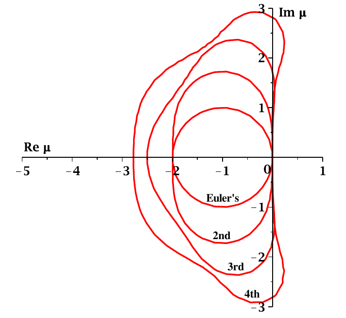
Specifically for Euler’s method, we have \(Q(\mu)=1+\mu\), and \(\mathcal{R}\) is a disc with center \(-1\) and radius \(1\). For higher-order Taylor methods, the regions of stability can be computed similarly; they are shown in Figure 10.2. For all examples of Runge-Kutta methods discussed in Section 10.6, the region agrees with that of the Taylor method of the same order. 6
However, from this picture, it appears that all of our methods are vulnerable to the problems posed by stiff equations, as suggested also by the example above. For having a stable method for a large range of step sizes, we need to look at a different approach. It turns out that certain implicit multi-step methods provide an advantage here.
Let us, in particular, consider the Implicit Trapezoidal method, which is given by the difference equation \[ \begin{split} \mathbf{w}_0&:=\boldsymbol{\alpha}, \\ \mathbf{w}_{i+1} &= \mathbf{w}_i + \frac{h}{2} (\mathbf{f}(x_{i+1},\mathbf{w}_{i+1}) + \mathbf{f}(x_i,\mathbf{w}_i)). \end{split} \tag{10.161}\] Applying it to the test equation Eq. 10.155, we obtain \[ w_{i+1} = w_i + \frac{h}{2} (\lambda w_{i+1} + \lambda w_i) = \big( 1 + \frac{\lambda h}{2} \big) w_i + \frac{\lambda h}{2} w_{i+1}. \tag{10.162}\] We can solve this for \(w_{i+1}\): \[ w_{i+1} = \frac{2+\lambda h}{2-\lambda h} w_i. \tag{10.163}\] Thus, the result is again of the form Eq. 10.159, with \[ Q(\mu) = \frac{2+\mu}{2-\mu}. \tag{10.164}\] Since \[ \begin{gathered} |Q(\mu)| < 1 \quad \Leftrightarrow \quad |2+\mu|^2 < |2-\mu|^2 \\ \quad \Leftrightarrow \quad 4+ 4 \mathop{\mathrm{Re}}\mu + |\mu|^2 < 4- 4 \mathop{\mathrm{Re}}\mu + |\mu|^2 \quad \Leftrightarrow \quad \mathop{\mathrm{Re}}\mu < 0, \end{gathered} \tag{10.165}\] the region of stability \(\mathcal{R}\) is just the left half plane. This is the maximum we could hope for: the implicit trapezoidal method gives reasonable results on stiff problems for all step sizes.
Methods of this kind, i.e., whose region of stability \(\mathcal{R}\) contains the entire left half plane, are called absolutely stable or A-stable.
One can apply the above stability analysis to other implicit methods as well, with some added complication – namely, when solving the difference equation as in Eq. 10.163, we may in general find several solutions. Figure 10.3 show the resulting regions of stability in some examples. Not all implicit methods are A-stable. In fact, there are no A-stable multistep methods of order \(O(h^3)\) or above. Sometimes, one uses a class of implicit multistep methods known as backward differentiation methods (BDM), which exist for arbitrary error order and come at least close to A-stability; we do not discuss them here.
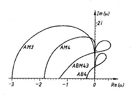
10.9.2 Implementing the Implicit Trapezoidal Method
Our analysis so far suggests that we should use the Implicit Trapezoidal method for the numerical treatment of stiff ODEs. However, since the difference equation of the method defines \(w_{i+1}\) only implicitly, this poses conceptual problems.
In the extremely simple case of the test equation Eq. 10.155, we were able to solve the difference equation explicitly for \(w_{i+1}\); see Eq. 10.163. We can generalize this to the case of a linear ODE: \[ y'(x) = \ell(x) y(x) + g(x), \quad a \leq x \leq b, \quad y(a)=\alpha. \tag{10.166}\]
Here \(\ell,g\) are continuous functions from \([a,b]\) to \(\mathbb{R}\). In this case, the difference equation Eq. 10.161 of the implicit trapezoidal method reads, \[ w_{i+1} = w_i + \frac{h}{2} \Big( \ell(x_{i+1}) w_{i+1} + g(x_{i+1}) +\ell(x_{i}) w_{i} + g(x_{i}) \Big). \tag{10.167}\] Much like in Eq. 10.163, this can be solved for \(w_{i+1}\): \[ \begin{gathered} w_{i+1} \Big( 1 - \frac{h}{2}\ell(x_{i+1}) \Big) = \Big( 1 + \frac{h}{2}\ell(x_{i}) \Big) + \frac{h}{2} g(x_{i+1})+ \frac{h}{2} g(x_{i}) % \\ \Rightarrow \quad w_{i+1} = \frac{2 + h \ell(x_{i})}{ 2 - h \ell(x_{i+1})} w_i + h \frac{g(x_{i+1}) + g(x_{i}) }{2 - h \ell(x_{i+1})}. \end{gathered} \tag{10.168}\] Thus, for linear ODEs as in Eq. 10.166, the implicit trapezoidal method can be applied with an explicit difference equation.
For a nonlinear ODE, it will generally not be possible to solve the difference equation symbolically. However, we can try to solve it numerically. As an approach for numerically solving nonlinear equations, we shall use Newton Iteration.
As a reminder: 7 Let \(F: \mathbb{R} \to \mathbb{R}\) be twice differentiable; suppose we are looking for a solution \(x\) of the equation \[ F(x) = 0. \tag{10.169}\] This solution is found with Newton’s method as follows. Starting with \(x_0\) sufficiently close to a solution, one recursively defines the sequence \[ x_k := x_{k-1} - \frac{F(x_{k-1})}{F'(x_{k-1})}. \tag{10.170}\] Then \(x_k \to x_\infty\) with \(F(x_\infty)=0\).
When implementing this on a computer, one cannot pass to the limit \(k \to \infty\), but needs to stop the iteration when a sufficient precision is reached. In practice, one usually takes the magnitude of the difference term on the r.h.s. of Eq. 10.170 as an indicator: The iteration is stopped when \(|F(x_{k-1})/F'(x_{k-1})|<T\), where \(T>0\) is the desired tolerance level.
In our situation of the implicit trapezoidal method, we need to solve the equation \[ w_{i+1} = w_i + \frac{h}{2} \big( f(x_i,w_i)+ f(x_{i+1},w_{i+1})\big). \tag{10.171}\] for \(w_{i+1}\), where \(x_i\), \(x_{i+1}\), \(w_i\) are given numbers. In other words, we are looking for zeros of the function \[ F(\hat{w}) = \hat{w} - w_i - \frac{h}{2} \big( f(x_i,w_i)+ f(x_{i+1},\hat{w})\big). \tag{10.172}\] Following Eq. 10.170, the following sequence should converge to the solution \(w_{i+1}\): \[ \begin{aligned} \hat{w}_0 &:= w_{i},\\ \hat{w}_k &:= \hat{w}_{k-1} - \underbrace{\frac{\hat{w}_{k-1} - w_i - \frac{h}{2}\big( f(x_i,w_i) + f(x_{i+1},\hat{w}_k) \big)}{ 1 - \frac{h}{2} \frac{\partial f}{\partial y}(x_{i+1},\hat{w}_{k-1}) }}_{=:v}. \end{aligned} \tag{10.173}\] We would run this iteration until \(|v|<T\).
Both in the case of linear and nonlinear equations, we have so far discussed a single ODE only. For applications in practice, we would need to generalize the methods to systems of ODEs. This is indeed possible, but requires a bit of thought.
In the linear case Eq. 10.166, one would consider a matrix-valued function \(\ell\) and a vector-valued \(g\). The difference equation can then still be solved symbolically, like in Eq. 10.168; however, the division by the factor \((2-h\ell(x_{i+1}))\) needs to be replaced by a multiplication with an inverse matrix, or equivalently, by solving a system of linear equations. Likewise, in the nonlinear case, we can handle ODE systems but would need the multi-dimensional version of Newton’s method (or, in other words, Newton’s method for systems of nonlinear equations). We shall not discuss the details of this generalization here.
The same example is considered in (Burden and Faires 2010, sec. 5.3).↩︎
The names of methods may vary in the literature; it is best to compare the tableaux when reading different sources!↩︎
If you hear someone speaking of “the Runge-Kutta method”, they are probably referring to this \(O(h^4)\) method.↩︎
This is not necessarily a realistic assumption - but one that simplifies the proof. One can do a similar argument using local bounds on \(\mathbf{f}\) and its derivatives in a suitable neighbourhood of the exact solution; however, this introduces formal complications which we want to avoid here.↩︎
We will not deal with any “global” error behaviour here.↩︎
This is true for all of our examples, but not for all Runge-Kutta methods in general.↩︎
For more details on Newton’s method for solving (single) nonlinear equations, see Section 3.5, or (Burden and Faires 2010, sec. 2.3).↩︎