In our digital age, mathematics isn’t just an abstract pursuit; it’s an essential tool that powers a vast array of applications. From weather forecasting to black hole simulations, from urban planning to medical research, the application of mathematics has become indispensable. Central to this applied force is Numerical Analysis.
Numerical Analysis is the discipline that bridges continuous mathematical theories with their concrete implementation on digital computers. These computers, by design, work with discrete quantities, and translating continuous problems into this discrete realm isn’t always straightforward. So why should you want to venture into Numerical Analysis?
Precision and Stability: Computers, despite their power, can introduce significant errors if mathematical problems are implemented without care. Numerical Analysis offers techniques to ensure we obtain results that are both accurate and stable.
Efficiency: Real-world applications often demand not just correctness, but efficiency. By grasping the methods of Numerical Analysis, we can design algorithms that are both accurate and resource-efficient.
Broad Applications: Whether your interest lies in physics, engineering, biology, finance, or many other scientific fields, Numerical Analysis provides the computational tools to tackle complex problems in these areas.
Basis for Modern Technologies: Core principles of Numerical Analysis are foundational in emerging fields such as artificial intelligence, quantum computing, and data science.
In this module, we’ll explore the key techniques, algorithms, and principles of Numerical Analysis that enable us to translate mathematical problems into computational solutions. We’ll delve into the challenges that arise in this translation, the strategies to overcome them, and the interaction of theory and practice.
By the end, you won’t merely understand the methods of scientific computing; you’ll be equipped to apply them efficiently and effectively in diverse scenarios. With a strong foundation in Numerical Analysis, you’ll be better prepared to engage with the practical challenges of the modern world.
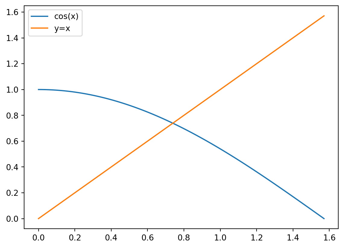
The main topic of this module is finding approximate solutions to various mathematical problems. A typical example for such a problem would be to find \(x>0\) such that \(\cos(x)=x\).
Code
# plot the function cos(x) and the line y=ximport numpy as npimport matplotlib.pyplot as plt# Define the range for x valuesx = np.linspace(0, np.pi/2, 100)# Plot cos(x)plt.plot(x, np.cos(x), label='cos(x)')# Plot y = xplt.plot(x, x, label='y=x')# Adding a legendplt.legend()
Figure 1.1
There is indeed one and only one such \(x\); this is apparent from a graph (Figure 1.1), and can also be proven rigorously without too much difficulty. However, it seems impossible to find a closed form expression for this \(x\): It’s not a fraction, a square root of a fraction, an integer multiple of \(\pi\), etc. For practical purposes, the best we can give is a numerical approximation of this \(x\), that is, we can compute it to, say, 10 decimal digits of accuracy.
This situation is pervasive in mathematics and its applications. Many problems of practical importance can be solved only approximately, and for others an approximation is much more efficient to find than the closed-form expression.
In Numerical Analysis, we aim to find approximation algorithms for mathematical problems, i.e., schemes that allow us to compute the solution approximately. These algorithms use only elementary operations (\(+,-,\times,/\)) but often a long sequence of them, so that in practice they need to be run on computers. This part of the problem—how to implement such algorithms on a computer—is called Scientific Computing.