7 Numerical integration

We now discuss approximation algorithms for evaluating definite integrals. For many functions of practical relevance, their antiderivative is not explicitly known, so that integrating them is not possible in explicit terms. For example, an integral like \[ \int_0^2 \exp(-x^2)dx \tag{7.1}\] can be evaluated only by numerical approximation.

The basic method for approximating an integral of a function \(f(x)\) is called numerical quadrature and uses a formula of the form \[ \int_a^bf(x)dx\approx \sum_{i=0}^nc_if(x_i), \tag{7.2}\] where \(x_0,\ldots,x_n\) are nodes and \(c_0,\ldots,c_n\) are weights. The nodes are chosen in the interval \([a,b]\) and the weights are chosen so that the formula is exact for polynomials of degree \(n\). The integral of a general function \(f\) is then approximated by the integral of the interpolating polynomial \(P_n\) of degree \(n\) through the nodes \(x_0,\ldots,x_n\) of \(f\). In other words, the integral is replaced with a discrete sum of function values of \(f\) with certain numerical coefficients.

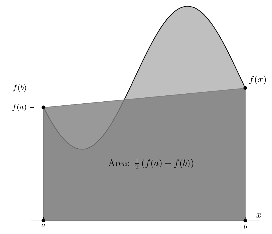
For a simple example, consider \(\int_a^bf(x)dx\) for a nonnegative function \(f\); illustrated in Figure 7.1. The integral \(\int_a^bf(x)dx\) corresponds to the area under the graph of \(f\) in the interval \([a,b]\). This region can be approximated by a trapezium through the points \((a,0)\), \((a,f(a))\), \((b,f(b))\), \((b,0)\). Computing the area of the trapezium, we obtain \[ \int_a^bf(x)dx\approx (b-a)\frac{(f(a)+f(b))}{2}. \tag{7.3}\] This is the so-called Trapezium rule.

We motivated the Trapezium rule geometrically, but two question remain open at this point:

How large is the approximation error?
How can the approximation be improved for additional precision?

We will answer these questions by generalizing the Trapezium rule as follows. First, we select a collection of distinct points \(x_0, x_1, \ldots, x_n\) from the interval \([a,b]\). Then, in generalization of the straight line that interpolated the function \(f\) in the Trapezium method, we construct the Lagrange interpolating polynomial (see Theorem 6.3) through \(x_0,\ldots,x_n\) to obtain \[ f(x)=\sum_{i=0}^nf(x_i)L_i(x) + R(x), \tag{7.4}\] where \[ R(x) = \frac{f^{(n+1)}(\xi(x))}{(n+1)!}\prod_{i=0}^n (x-x_i) \tag{7.5}\] and \(\xi(x)\in[a,b]\) for each \(x\). Integrating this formula over \([a, b]\), we obtain \[ \int_a^bf(x)dx=\sum_{i=0}^nc_if(x_i) + E(f) \tag{7.6}\] where \[ \begin{aligned} c_i&= \int_a^b L_i(x)dx, & E(f)&=\int_a^b R(x)\,dx. \end{aligned} \tag{7.7}\] The idea is that it is desirable for the error term \(E(f)\) to be small—more on that below.

It is usual to choose the nodes \(x_0,\ldots,x_n\) equally spaced in the interval \([a,b]\), in other words, with \(h=\frac{1}{n}(b-a)\), one sets \[ x_i := a + i h \quad\text{for }i=0,\ldots,n. \tag{7.8}\] The construction above then yields the so called closed Newton-Cotes formulae for integration. Let us consider the cases of \(n=1\) (which corresponds to the Trapezium rule as above) and \(n=2\) in more detail.

7.1 Trapezium rule

Let us now put \(n=1\), that is, we use interpolation by a straight line. Following the recipe from above, we have \(h:=b-a\), the nodes are \(x_0=a\) and \(x_1=b\), and we have the Lagrange polynomials \[ \begin{split} L_0(x) &= \frac{x-x_1}{x_0-x_1} = -\frac{1}{h}(x-b), \\ L_1(x) &= \frac{x-x_0}{x_1-x_0} = \frac{1}{h}(x-a). \end{split} \tag{7.9}\] The constants \(c_0,c_1\) are then \[ \begin{split} c_0 &= \int_a^b L_0(x) dx = -\frac{1}{h}\int_a^b (x-b) dx \\ &= -\frac{1}{2h}\left[(x-b)^2\right]_{x=a}^b = \frac{h}{2},\\ c_1 &= \int_a^b L_1(x) dx = \frac{1}{h}\int_a^b (x-a) dx \\ &= \frac{1}{2h}\left[(x-a)^2\right]_{x=a}^b = \frac{h}{2}. \end{split} \tag{7.10}\] The approximation formula Eq. 7.6 then gives \[ \int_a^bf(x)dx \approx \frac{h}{2}(f(a)+f(b)), \tag{7.11}\] which is exactly the Trapezium rule.

Remark. It can be shown by direct calculation that the Trapezium rule produces an exact result for \(f(x)=1\), \(f(x)=x\) and, hence for any polynomial of degree \(0\) and \(1\). (Prove it!)

Let us now consider the error term \(E(f)\). We assume that \(f\in C^{2}[a,b]\) and employ the formula for the error of the interpolation polynomial \[ f(x)=P(x)+\frac{f^{\prime\prime}(\xi(x))}{2!}(x-x_{0})(x-x_{1}). \tag{7.12}\] Since \(f\in C^{2}[a,b]\), we have \[ m\leq f^{\prime\prime}(x)\leq M \quad \text{ for \ all } \ \ x\in[a,b], \tag{7.13}\] where \[ m=\min_{x\in[a,b]} f^{\prime\prime}(x), \quad M=\max_{x\in[a,b]} f^{\prime\prime}(x) . \tag{7.14}\] Let \[ B(x)=-\frac{(x-x_{0})(x-x_{1})}{2}. \tag{7.15}\] Evidently, \(B(x)\geq 0\) for all \(x\in[a,b]\). Therefore, it follows from Eq. 7.12 that \[ m \, B(x) \leq P(x)-f(x) \leq M \, B(x). \tag{7.16}\] Integration of these inequalities yields \[ m \, \int_{x_{0}}^{x_{1}} B(x)dx \leq \int_{x_{0}}^{x_{1}}\left(P(x)-f(x)\right)dx \leq M \, \int_{x_{0}}^{x_{1}}B(x)dx. \tag{7.17}\] Since \[ \begin{split} \int_{x_{0}}^{x_{1}} B(x)dx &=\frac{1}{2}\int_{x_{0}}^{x_{1}}(x-x_{0})(x_{1}-x)dx \\ &=\frac{1}{2}\int_{0}^{1}h \, t \, h (1-t) \, h \, dt\\ &=\frac{h^3}{2}\left(\frac{t^2}{2}-\frac{t^3}{3}\right)\Biggm\vert_{t=0}^{t=1}=\frac{h^3}{12}. \end{split} \tag{7.18}\] (here we have introduced new variable of integration \(t\) by the formula \(x=x_{0}+t h\)) Eq. 7.17 can we rewritten as \[ m \leq \frac{12}{h^3}\int_{x_{0}}^{x_{1}}\left(P(x)-f(x)\right)dx \leq M . \tag{7.19}\] Since \(f^{\prime\prime}(x)\) is continuous in \([a,b]\), the intermediate value theorem says that there exists \(\xi\in[a,b]\) such that \[ f^{\prime\prime}(\xi)=\frac{12}{h^3}\int_{x_{0}}^{x_{1}}\left(P(x)-f(x)\right)dx. \tag{7.20}\] This and the expression for the integral of \(P(x)\) give us the Trapezium rule with error term: \[ \int_{x_{0}}^{x_{1}}f(x)dx = \frac{h}{2}\left(f(x_{0})+f(x_{1})\right)-\frac{h^3}{12}f^{\prime\prime}(\xi). \tag{7.21}\] We see that the error term can be controlled by an estimate of the second derivative of \(f\). Also, it will be small if \(h\) is small. Evidently, for a fixed interval \([a,b]\) we cannot vary \(h\) to reduce the error; we will return to this problem later.

7.2 Simpson’s rule

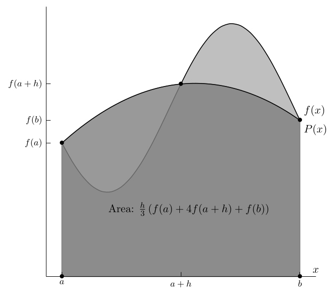
Now let us consider the case \(n=2\), which should yield a better approximation. We have \(h=\tfrac{1}{2}(b-a)\), and our nodes are \(x_0=a\), \(x_1=a+h\), \(x_2=a+2h=b\). We first recall the polynomials \(L_j\): \[ \begin{split} L_0(x) &= \frac{(x-x_1)(x-x_2)}{(x_0-x_1)(x_0-x_2)}=\frac{1}{2h^2}(x-(a+h))(x-b), \\ L_1(x) &= \frac{(x-x_0)(x-x_2)}{(x_1-x_0)(x_1-x_2)}=-\frac{1}{h^2}(x-a)(x-b), \\ L_2(x) &= \frac{(x-x_0)(x-x_1)}{(x_2-x_0)(x_2-x_1)}=\frac{1}{2h^2}(x-a)(x-(a+h)). \end{split} \tag{7.22}\] Their integrals are, with the same substitution \(x=a+ht\) as before (but now \(0 \leq t \leq 2\)), \[ \begin{split} c_0=\int_a^b L_0(x)\,dx &= \frac{h}{2} \int_0^2 (t-1)(t-2) dt = \frac{h}{2}\frac{2}{3} = \frac{h}{3}, \\ c_1=\int_a^b L_1(x)\,dx &= -h \int_0^2 t(t-2) dt = -h\left( -\frac{4}{3}\right) = \frac{4h}{3}, \\ c_2=\int_a^b L_2(x)\,dx &= \frac{h}{2} \int_0^2 t(t-1) dt = \frac{h}{2}\frac{2}{3} = \frac{h}{3}. \end{split} \tag{7.23}\] This means that our approximation formula is \[ \int_a^bf(x)dx \approx \frac{h}{3}\left( f(a)+4 f(a+h)+f(b)\right). \tag{7.24}\] This is known as Simpson’s rule, which is graphically represented in Figure 7.2.

Error term for Simpson’s rule. Let us recall the Trapezium rule with error term: \[ \int_{x_{0}}^{x_{1}}f(x)dx = \frac{h}{2}\left[f(x_{0})+f(x_{1})\right]- \frac{h^3}{12}f^{\prime\prime}(\xi). \tag{7.25}\] It has been obtained by integrating the linear interpolating polynomial with nodes \(x_{0}\) and \(x_{1}=x_{0}+h\). Therefore, it must produce an exact result for any polynomial of degree 0 and 1. Indeed, the error term in Eq. 11.59 vanishes for polynomials of degree 0 and 1.

Simpson’s rule has been obtained by integrating the quadratic interpolating polynomial with nodes \(x_{0}\), \(x_{1}=x_{0}+h\) and \(x_{2}=x_{0}+2h\). So, it must produce an exact result for polynomials of degree 0, 1 and 2. Will it generate a nonzero error for cubic polynomials? To examine this, it suffices to consider \(f(x)=x^3\). By analogy with the Trapezium rule we assume that Simpson’s rule with error term has the form \[ \int_{x_{0}}^{x_{2}}f(x)dx = \frac{h}{3}\left[f(x_{0})+4f(x_{1}) + f(x_{2})\right] +Cf'''(\xi) \tag{7.26}\] for some constant \(C\) and some \(\xi\in[x_{0},x_{2}]\). Substituting \(f(x)=x^3\) in Eq. 7.26, we obtain \[ \int_{x_{0}}^{x_{2}}x^3 dx = \frac{h}{3}\left[x_{0}^3+4x_{1}^3 + x_{2}^3\right] +6C. \tag{7.27}\] The integral on the left hand side of Eq. 11.69 can be written as \[\begin{split} (\text{ l.h.s. }) \, &= \, \frac{x_{2}^{4}}{4}-\frac{x_{0}^{4}}{4} =\frac{(x_{0}+2h)^{4}}{4}-\frac{x_{0}^{4}}{4}\\ &=2h x_{0}^{3}+6h^2 x_{0}^{2}+8h^3 x_{0}+4h^4. \end{split} \tag{7.28}\] For the right hand side of Eq. 11.69, we have \[ \begin{split} (\text{ r.h.s. }) &=\frac{h}{3}\left[x_{0}^3+4(x_{0}+h)^3 + (x_{0}+2h)^3\right]+6C \\ &=\frac{h}{3}\Bigl[x_{0}^3+4\left(x_{0}^{3}+3x_{0}^{2}h+3x_{0}h^{2}+h^{3}\right)\\ &\qquad\qquad + x_{0}^{3}+6x_{0}^{2}h+12x_{0}h^{2}+8h^{3}\Bigr]+6C\\ &=\frac{h}{3}\left[6x_{0}^3+18x_{0}^{2}h+24x_{0}h^{2}+12h^{3}\right]+6C\\ &=2h x_{0}^{3}+6h^2 x_{0}^{2}+8h^3 x_{0}+4h^4+6C. \end{split} \tag{7.29}\] If follows from Eq. 7.28 and Eq. 7.29 that Eq. 11.69 simplifies to \(0=6C\), so that \(C=0\). This means that Simpson’s rule is exact for polynomials of degree 3 (an unexpected result!).

This also means that our assumption about the error term for Simpson’s rule is wrong. So, we make another assumption, namely: \[ \int_{x_{0}}^{x_{2}}f(x)dx = \frac{h}{3}\left[f(x_{0})+4f(x_{1}) + f(x_{2})\right] +Cf^{(4)}(\xi). \tag{7.30}\] To find \(C\), we substitute \(f(x)=x^4\) in Eq. 7.30. This yields the equation \[ \int_{x_{0}}^{x_{2}}x^4 dx = \frac{h}{3}\left[x_{0}^4+4x_{1}^4 + x_{2}^4\right] +24C. \tag{7.31}\] The left hand side of Eq. 7.31 can be written as \[\begin{split} (\text{ l.h.s. }) \, &= \, \frac{x_{2}^{5}}{5}-\frac{x_{0}^{5}}{5} =\frac{(x_{0}+2h)^{5}}{5}-\frac{x_{0}^{4}}{4}\\ &=2h x_{0}^{4}+8h^2 x_{0}^{3}+16h^3 x_{0}^{2}+16h^4 x_{0}+\frac{32}{5}h^5. \end{split} \tag{7.32}\] For the right hand side of Eq. 7.31, we have \[ \begin{split} (\text{ r.h.s. }) &=\frac{h}{3}\left[x_{0}^4+4(x_{0}+h)^4 + (x_{0}+2h)^4\right]+24C\\ &=\frac{h}{3}\Bigl[x_{0}^3+4\left(x_{0}^{4}+4x_{0}^{3}h+6x_{0}^{2}h^2 + 4x_{0}h^3 +h^{4}\right)\\ & \qquad\qquad + x_{0}^{4}+8x_{0}^{3}h+24x_{0}^{2}h^2+ 32x_{0}h^{3}+16h^{4}\Bigr]+24C\\ &=\frac{h}{3}\left[6x_{0}^4+24x_{0}^{3}h+48x_{0}^{2}h^{2}+48x_{0}h^{3}+20h^{4}\right]+24C\\ &=2h x_{0}^{4}+8h^2 x_{0}^{3}+16 h^3 x_{0}^{2}+16 h^4 x_{0}+\frac{20}{3}h^5+24C. \end{split} \tag{7.33}\] Eq. 7.31–Eq. 7.33 imply that \[ \frac{32}{5}h^5=\frac{20}{3}h^5+24C. \tag{7.34}\] so that \[ C=-\frac{h^5}{90}. \tag{7.35}\] Thus, Simpson’s rule with error term is given by \[ \int_{x_{0}}^{x_{2}}f(x)dx = \frac{h}{3}\left[f(x_{0})+4f(x_{1}) + f(x_{2})\right] -\frac{h^{5}}{90}f^{(4)}(\xi) \tag{7.36}\] for some \(\xi\in[x_{0},x_{2}]\). Note that the above argument is not a proof of the existence of such \(\xi\). Alternative derivations of formula Eq. 7.36 can be found in textbooks on Numerical Analysis (e.g. (Burden and Faires 2010)).

7.3 Higher-order Newton-Cotes formulae

We have now seen that the Trapezium and Simpson’s rules are examples of Newton-Cotes formulae, which are obtained by integrating of an interpolating polynomial for interpolation points \(x_{0}, \dots, x_{n}\). The Trapezium rule and Simpson’s rule correspond to \(n=1\) and \(n=2\) respectively. For \(n=3\), we have Simpson’s three-eighth rule \[ \int_{x_{0}}^{x_{3}}f(x)dx= {3h \over 8} \left[f(x_{0})+3f(x_{1})+3f(x_{2})+f(x_{3})\right]- {3h^{5} \over 80}f^{(4)}(\xi), \tag{7.37}\] where \(h=(x_{3}-x_{0})/3\) and \(\xi\in[x_{0},x_{3}]\). The error of Simpson’s three-eighth rule is proportional to \(h^5\) with a coefficient that is larger than that in the error term of Simpson’s rule, so this method seems less efficient than Simpson’s rule.

For \(n=4\) we have the formula \[ \begin{split} \int_{x_{0}}^{x_{4}}f(x)dx=& {2h \over 45} \left[7f(x_{0})+32f(x_{1})+12f(x_{2})+32f(x_{3}) +7f(x_{4})\right]\\ &-{8h^{7} \over 945}f^{(6)}(\xi). \end{split} \tag{7.38}\] where \(h=(x_{4}-x_{0})/4\) and \(\xi\in[x_{0},x_{4}]\).

7.4 Composite numerical integration

The Newton-Cotes formulas are generally unsuitable for large integration intervals. This would require high-degree formulas. An alternative to this is a piecewise approach to numerical integration that uses the low-order Newton-Cotes formulas such as the Trapezium and Simpson’s rules.

Let us apply Simpson’s formula to approximate the integral \(\int_{0}^{4}x^{4}dx\). We have \[ \begin{split} I &= \int_{0}^{4}x^{4}dx\approx \frac{2}{3} \left[0 + 4\cdot 2^{4}+4^{4}\right]=\frac{2}{3}(64+256)=213.333, \\ E&=\vert I-213.333\vert=\vert 204.8-213.333\vert=8.533. \end{split} \tag{7.39}\] To apply a piecewise technique to this problem, we divide \([0, 4]\) into two subintervals \([0, 2]\) and \([2, 4]\) and use Simpson’s rule twice with \(h=1\): \[ \begin{split} I =& \int_{0}^{4}x^{4}dx\approx \frac{1}{3} \left[0 + 4\cdot 1^{4}+2^{4}\right] \\ &+ \frac{1}{3}\left[2^{4} + 4\cdot 3^{4}+4^{4}\right]=205.333, \\ E=&\vert 204.8-205.333\vert=0.533. \end{split} \tag{7.40}\] To reduce the error, we can proceed further by subdividing the intervals \([0, 2]\) and \([2, 4]\) and use Simpson’s rule with \(h=1/2\).

To generalize this procedure, we choose an even integer \(n\) and divide the interval \([a, b]\) into \(n\) subintervals. Then we apply Simpson’s rule to each consecutive pair of subintervals. With \(h=(b-a)/n\) and \(x_{j}=a+jh\) for \(j=0, 1, ..., n\), we have \[ \begin{split} \int_{a}^{b}f(x)dx &=\sum_{j=1}^{n/2} \int_{x_{2j-2}}^{x_{2j}}f(x)dx \\ &= \sum_{j=1}^{n/2}\left\{ \frac{h}{3}\left[f(x_{2j-2})+4f(x_{2j-1})+f(x_{2j})\right]- \frac{h^{5}}{90}f^{(4)}(\xi_{j})\right\} \end{split} \tag{7.41}\] for some \(\xi_{j}\) between \(x_{2j-2}\) and \(x_{2j}\), provided that \(f\in C^{4}[a, b]\).

One can see that for each \(j=1, 2, ..., (n/2)-1\), the number \(f(x_{2j})\) appears in the term corresponding to the interval \([x_{2j-2}, x_{2j}]\) and also in the term corresponding to the interval \([x_{2j}, x_{2j+2}]\). Taking this into account, we obtain \[ \begin{split} \int_{a}^{b}f(x)dx &= \sum_{j=1}^{n/2} \int_{x_{2j-2}}^{x_{2j}}f(x)dx \\ &= \frac{h}{3}\left\{ f(x_{0})+2\sum_{j=1}^{(n/2)-1}f(x_{2j})+ 4\sum_{j=1}^{n/2}f(x_{2j-1})+ f(x_{n})\right\} +E. \end{split} \tag{7.42}\] The error of this approximation is \[ E=-{h^{5} \over 90}\sum_{j=1}^{n/2}f^{(4)}(\xi_{j}) \tag{7.43}\] where \(x_{2j-2} < \xi_{j} < x_{2j}\) for each \(j=1, 2, ..., n/2\). If \(f\in C^{4}[a, b]\), then (according to the Extreme Value Theorem) \(f^{(4)}(x)\) attains its maximum and minimum values in \([a, b]\). Let \[ m=\min_{x\in[a, b]}f^{(4)}(x), \quad M=\max_{x\in[a, b]}f^{(4)}(x). \tag{7.44}\] Then we have \[ m \leq f^{(4)}(\xi_{j}) \leq M \ \ \ \text{ for \ each } \ \ j=1, 2, ..., n/2 . \tag{7.45}\] Therefore, \[ \frac{n}{2}m \leq \sum_{j=1}^{n/2}f^{(4)}(\xi_{j}) \leq \frac{n}{2} M, \tag{7.46}\] and \[ m \leq \frac{2}{n} \sum_{j=1}^{n/2}f^{(4)}(\xi_{j}) \leq M. \tag{7.47}\] By the Intermediate Value Theorem, there is a \(\mu\in(a, b)\) such that \[ f^{(4)}(\mu)={2 \over n} \sum_{j=1}^{n/2}f^{(4)}(\xi_{j}). \tag{7.48}\] Hence, \[ E=-{h^{5}\over 180}n f^{(4)}(\mu)=-{b-a \over 180}h^{4} f^{(4)}(\mu). \tag{7.49}\] Thus, we have proved the following theorem.

Theorem 7.1 (Composite Simpson’s rule) Let \(f\in C^{4}[a, b]\), \(n\) be even, \(h=(b-a)/n\), and \(x_{j}=a+jh\) for \(j=0, 1, ..., n\). There exist a number \(\mu\in(a, b)\) such that \[ \begin{split} \int_{a}^{b}f(x)dx =& {h\over 3}\left\{ f(x_{0})+2\sum_{j=1}^{(n/2)-1}f(x_{2j})+ 4\sum_{j=1}^{n/2}f(x_{2j-1})+ f(x_{n})\right\} \\ &-\frac{b-a}{180}h^{4}f^{(4)}(\mu). \end{split} \tag{7.50}\]

Similarly, one can prove analogous theorems for Composite Trapezium rule.

Theorem 7.2 (Composite Trapezium rule) Let \(f\in C^{2}[a, b]\), \(h=(b-a)/n\), and \(x_{j}=a+jh\) for \(j=0, 1, ..., n\). There exist a number \(\mu\in(a, b)\) such that \[ \int_{a}^{b}f(x)dx= \frac{h}{2}\left\{ f(x_{0})+2\sum_{j=1}^{n-1}f(x_{j})+ f(x_{n})\right\} -\frac{b-a}{12}h^{2}f^{\prime\prime}(\mu). \tag{7.51}\]

Example 7.1 Apply the composite Simpson rule to compute \[ I=\int\limits_{0}^{2}e^{x}dx \tag{7.52}\] with absolute error less than \(10^{-2}\).

Solution. First we need to determine the number of subintervals* \(n\) in the composite Simpson rule that would ensure that absolute error less than \(10^{-2}\). It follows from Eq. 7.50 that \[ E=\frac{b-a}{180}h^{4}\vert f^{(4)}(\mu)\vert\leq \frac{b-a}{180}h^{4}M, \tag{7.53}\] where \(M\) is the upper bound for \(\vert f^{(4)}(x)\vert\) in \([0,2]\). Evidently, \(M=e^2\). Therefore, we require that \[ \frac{b-a}{180}h^{4}e^2 < 10^{-2} \quad \Leftrightarrow \quad \frac{(b-a)^5}{180 n^4}e^2 < 10^{-2} \quad \Leftrightarrow \quad n^4 > \frac{100(b-a)^5}{180}e^2 . \tag{7.54}\] Substituting \(a=0\) and \(b=2\), we find that \[ n^4 > \frac{5\cdot 32 e^2}{9}=131.3609973, \quad \text{ so \ that } \ \ n\geq 4 \ \ (n^4=256). \tag{7.55}\] Applying the composite Simpson rule with \(n=4\), we obtain the approximation \[ \tilde{I}=6.391210187. \tag{7.56}\] The actual error is \[ \vert I-\tilde{I}\vert=0.002154088. \tag{7.57}\] So it is indeed less that \(10^{-2}\).

All the Composite Newton-Cotes techniques are stable with respect to roundoff error. Consider, for example, the Composite Simpson rule with \(n\) subintervals applied to a function \(f(x)\) on \([a, b]\). We assume that \(f(x_{i})\) is approximated by \(\tilde f(x_{i})\) with the roundoff error \(e_{i}\). Then, the accumulated error in the Composite Simpson rule is \[ \begin{split} E(h) &= \left\vert\frac{h}{3}\left( e_{0} +2\sum_{j=1}^{(n/2)-1}e_{2j}+ 4\sum_{j=1}^{n/2}e_{2j-1}+ e_{n}\right)\right\vert \\ &\leq \frac{h}{3}\left( \vert e_{0}\vert +2\sum_{j=1}^{(n/2)-1}\vert e_{2j}\vert + 4\sum_{j=1}^{n/2}\vert e_{2j-1}\vert + \vert e_{n}\vert\right) \end{split} \tag{7.58}\] If the roundoff errors are uniformly bounded by \(\varepsilon\), then \[ E(h) \leq {h \over 3}\left(\varepsilon +2\left(\frac{n}{2}-1\right)\varepsilon + 4\frac{n}{2}\varepsilon + \varepsilon\right)=nh\varepsilon=(b-a)\varepsilon. \tag{7.59}\] Thus, the bound for the accumulated error is independent of \(h\), so that \(h\) can be taken as small as we wish.