Code
import numpy as np
import matplotlib.pyplot as plt
f = lambda x: (np.sin(4*x)+1)*((x-5)**2-25)
x = np.linspace(0,8,100)
plt.plot(x,f(x))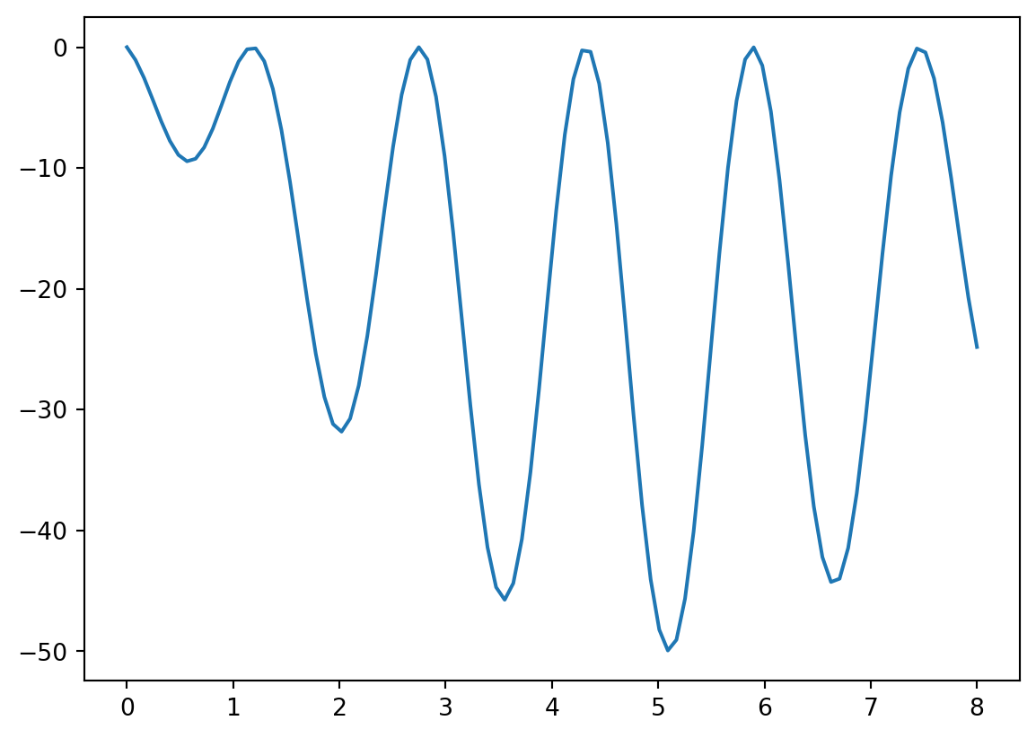
It is not enough to do your best; you must know what to do, and then do your best.
–W. Edwards Deming
In applied mathematics we are often not interested in all solutions of a problem but in the optimal solution. Optimization therefore permeates many areas of mathematics and science. In this section we will look at a few examples of optimization problems and the numerical methods that can be used to solve them.
Exercise 5.1 Here is an atypically easy optimisation problem that you can quickly do by hand:
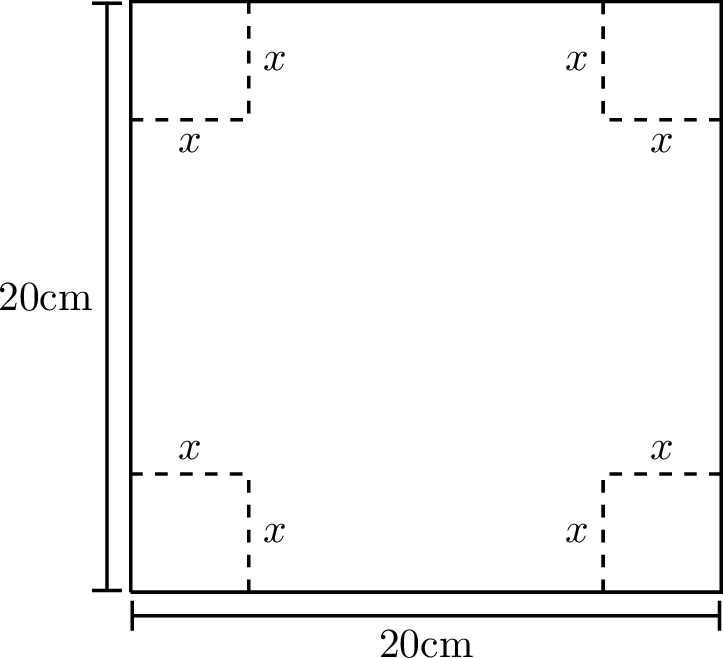
A piece of cardboard measuring 20cm by 20cm is to be cut so that it can be folded into a box without a lid (see Figure 5.1). We want to find the size of the cut, \(x\), that maximizes the volume of the box.
Write a function for the volume of the box resulting from a cut of size \(x\). What is the domain of your function?
We know that we want to maximize this function so go through the full Calculus exercise to find the maximum:
take the derivative
set it to zero
find the critical points
test the critical points and the boundaries of the domain using the extreme value theorem to determine the \(x\) that gives the maximum.
An optimization problem is approached by first writing the quantity you want to optimize as a function of the parameters of the model. In the previous exercise that was the function \(V(x)\) that gives the volume of the box as a function of the parameter \(x\), which was the length of the cut. That function then needs to be maximized (or minimized, depending on what is optimal).
Exercise 5.2 In the previous example it was easy to find the value of \(x\) that maximized the function analytically However, in many cases it is not so easy. The equation for the parameters that arises from setting the derivatives to zero is usually not solvable analytically. In these cases we need to use numerical methods to find the extremum. Take for example the function \[f(x) = e^{-x^2} + \sin(x^2)\] on the domain \(0 \le x \le 1.5\). The maximum of this function on this domain can not be determined analytically.
Use Python to make a plot of this function over this domain. You should get something similar to the graph shown in Figure 5.2. What is the \(x\) that maximizes the function on this domain? What is the \(x\) that minimizes the function on this domain?
import numpy as np
import matplotlib.pyplot as plt
x = np.linspace(0,1.5,100)
f = np.exp(-x**2) + np.sin(x**2)
plt.xlabel('$x$')
plt.ylabel('$f(x)$')
plt.plot(x,f)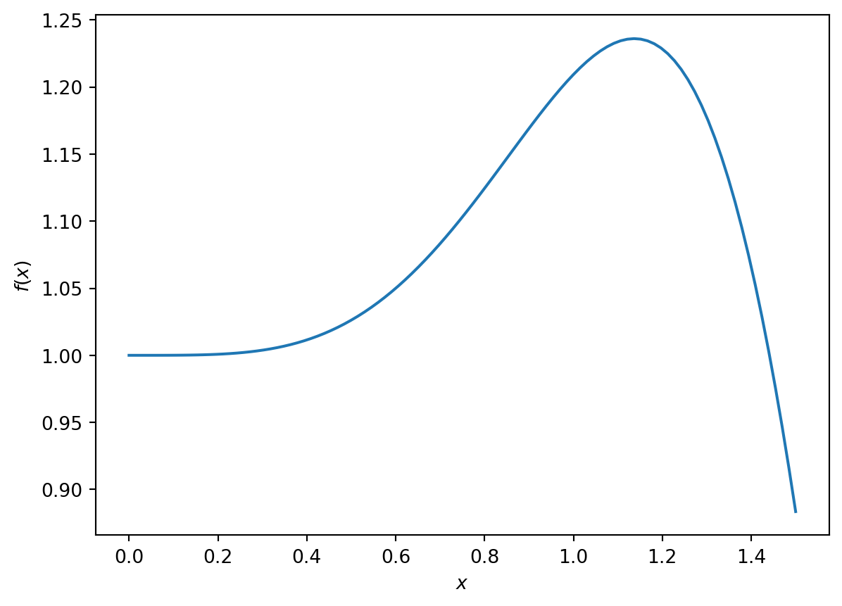
The intuition behind numerical optimization schemes is typically to visualize the function that you are trying to minimize or maximize and think about either climbing the hill to the top (maximization) or descending the hill to the bottom (minimization).
Exercise 5.3 If you were blind folded and standing on a hillside, could you find the top of the hill? (assume no trees and no cliffs …this is not supposed to be dangerous) How would you do it? Explain your technique clearly.
Exercise 5.4 If you were blind folded and standing on a crater on the moon could you find the lowest point? How would you do it? Remember that you can hop as far as you like … because gravity … but sometimes that’s not a great thing because you could hop too far.
Clearly there is no difference between finding the maximum of a function and finding the minimum of a function. The maximum of a function \(f\) is exactly at the same point as the minimum of the function \(-f\). For concreteness we will from now on focus on finding the minimum of a function.
The preceding thought exercises have given you intuition about finding extrema in a two-dimensional landscape. But first we will reduce back to one-dimensional optimization problems before generalising to multiple dimensions in the next section.
Exercise 5.5 Try to turn your intuitions into algorithms. If \(f(x)\) is the function that you are trying to minimize then turn your ideas from the previous exercises into step-by-step algorithms which could be coded. Then try out your codes on the function \[\begin{equation} f(x) = -e^{-x^2} - \sin(x^2) \end{equation}\] to see if your algorithms can find the local minimum near \(x \approx 1.14\). Try to generate several different algorithms.
One obvious method would be to simply evaluate the function at many points and choose the smallest value. This is called a brute force search.
import numpy as np
x = np.linspace(0,1.5,1000)
f = -np.exp(-x**2) - np.sin(x**2)
print(x[np.argmin(f)])
This method is not very efficient. Just think about how often you would need to evaluate the function for the above approach to give the answer to 12 decimal places. It would be a lot! Your method should be more efficient.
The advantage of this brute force method is that it is guaranteed to find the global minimum in the interval. Any other, more efficient method can get stuck in local minima.
Exercise 5.6 Here is an idea for a method that is similar to the bisection method for root finding.
In the bisection method we needed a starting interval so that the function values had opposite signs at the endpoints. You were therefore guaranteed that there would be at least one root in that interval. Then you chose a point in the middle of the interval and by looking at the function value at that new point were able to choose an appropriate smaller interval that was still guaranteed to contain a root. By repeating this you honed in on the root.
Unfortunately by just looking at the function values at two point there is no way of knowing whether there is a minimum between them. However, if you were to look at the function values at three points and found that the value at the middle point was less than the values at the endpoints then you would know that there was a minimum between the endpoints.
The idea now is to choose a new point between the two outer points, compare the function value there to those at the previous three points, and then choose a new triplet of points that is guaranteed to contain a minimum. By repeating this process you would hone in on the minimum.
Complete the following function to implement this idea. You need to think about how to choose the new point and then how to choose the new triplet.
def bracketing(f, a, b, c, tol = 1e-12):
    """
    Find an approximation of a local minimum of a function f within the
    interval [a, b] using a bracketing method.

    The function narrows down the interval [a, b] by maintaining a
    triplet (a, c, b) where f(c) < f(a) and f(c) < f(b).
    The process iteratively updates the triplet to home in on the minimum,
    stopping when the interval is smaller than `tol`.

    Parameters:
    f (function): A unimodal function to minimize.
    a, b (float): The initial interval bounds where the minimum is to be
                  searched. It is assumed that a < b.
    c (float): An initial point within the interval (a, b) where
               f(c) < f(a) and f(c) < f(b).
    tol (float): The tolerance for the convergence of the algorithm.
                 The function stops when b - a < tol.

    Returns:
    float: An approximation of a point where f achieves a local minimum.
    """

    # Check that the point are ordered a < c < b

    # Check that the function value at `c` is lower than at both `a` and `b`

    # Loop until you have an interval smaller than the tolerance
    while b-a > tol:

        # Choose a new point `d` between `a` and `b`
        # Think about what is the most efficient choice

        # Compare f(d) with f(c) and use the result
        # to choose a new triplet `a`, `b`, `c` in such a way that
        # b-a has decreased but f(c) is still lower than both f(a) and f(b)

        # While debugging, include a print statement to let you know what
        # is happening within your loop

    return c
Let us next explore the intuitive method of simply taking steps in the downhill direction. That should eventually bring us to a local minimum. The problem is only to know how to choose the step size and the direction. The gradient descent method is a simple and effective way to do this. By making the step be proportional to the negative gradient of the function we are guaranteed to be moving in the right direction and we are also automatically reducing the step size as we get closer to the minimum where the gradient gets smaller.
Let \(f(x)\) be the objective function which you are seeking to minimize.
Find the derivative of your objective function, \(f'(x)\).
Pick a starting point, \(x_0\).
Pick a small control parameter, \(\alpha\) (in machine learning this parameter is called the “learning rate” for the gradient descent algorithm).
Use the iteration \(x_{n+1} = x_n - \alpha f'(x_n)\).
Iterate (decide on a good stopping rule)
Exercise 5.7 What is the Gradient Ascent/Descent algorithm doing geometrically? Draw a picture and be prepared to explain to your peers.
Exercise 5.8 Write code to implement the 1D gradient descent algorithm and use it to solve Exercise 5.1. Compare your answer to the analytic solution.
def gradient_descent(df, x0, learning_rate,
                     tol = 1e-12, max_iter=10000):
    """
    Find an approximation of a local minimum of a function f
    using the gradient descent method.

    The function iteratively updates the current guess `x0`
    by moving in the direction of the negative gradient
    of `f` at `x0` by a distance `alpha`.
    The process stops when the magnitude of the gradient
    is smaller than `tol`.

    Parameters:
    df (function): The derivative of the function you
                   want to minimize.
    x0 (float): The initial guess for the minimum.
    learning_rate (float): The learning rate multiplies the
                           gradient to give the step size.
    tol (float): The tolerance for the convergence.
                 The function stops when |df(x0)| < tol.
    max_iter (int): The maximal number of iterations to perform.

    Returns:
    float: An approximation of a point where f achieves
           a local minimum.
    """
    # Initialize x with the starting value
    x = x0
    # Loop for a maximum of `max_iter` iterations
    for i in range(max_iter):
        # Calculate the step size by multiplying the learning
        # rate with the derivative at the current guess

        # Update `x` by adding the step

        # If the step size was smaller than `tol` then
        # return the new `x`

    # If the loop finishes without returning then print a
    # warning that the last step size was larger than `tol`.

    # Return the last `x` value
Exercise 5.9 Compare an contrast the methods you came up with in Exercise 5.5 with the methods proposed in Exercise 5.6 and Exercise 5.8.
What are the advantages to each of the methods proposed?
What are the disadvantages to each of the methods proposed?
Which method, do you suppose, will be faster in general? Why?
Which method, do you suppose, will be slower in general? Why?
Exercise 5.10 Make a plot of the log of the absolute error at iteration \(k+1\) agains the log of the absolute error at iteration \(k\), similar to Figure 3.5 for several methods and several choices of function. What do you observe?
Exercise 5.11 Try out your algorithms to find the minimum of the function \[f(x) = (\sin(4x)+1)((x-5)^2-25)\] on the domain \(0 \le x \le 8\).
import numpy as np
import matplotlib.pyplot as plt
f = lambda x: (np.sin(4*x)+1)*((x-5)**2-25)
x = np.linspace(0,8,100)
plt.plot(x,f(x))What do you observe?
Now let us look at multi-variable optimization. The idea is the same as in the single-variable case. We want to find the minimum of a function \(f(x_1, x_2, \ldots, x_n)\). Such higher-dimensional problems are very common and the dimension \(n\) can be very large in practical problems. A good example is the loss function of a neural network which is a function of the weights and biases of the network. In a large language model the loss function is a function of many billions of variables and the training of the model is a large optimization problem.
Here is a two-variable example: Find the minimum of the function \[f(x,y) = \sin(x)\exp\left(-\sqrt{x^2+y^2}\right)\]
import numpy as np
import plotly.graph_objects as go

f = lambda x, y: np.sin(x)*np.exp(-np.sqrt(x**2+y**2))

# Generating values for x and y
x = np.linspace(-2, 2, 100)
y = np.linspace(-1, 3, 100)

X, Y = np.meshgrid(x, y)
Z = f(X, Y)

# Creating the plot
fig = go.Figure(data=[go.Surface(z=Z, x=X, y=Y)])
fig.update_layout(width=800, height=800)Finding the minima of multi-variable functions is a bit more complicated than finding the minima of single-variable functions. The reason is that there are many more directions in which to move. But the basic intuition that we want to move downhill to move towards a minimum of course still works. The gradient descent method is still a good choice for finding the minimum of a multi-variable function. The only difference is that the gradient is now a vector and the step is in the direction of the negative gradient.
Exercise 5.12 In your group, answer each of the following questions to remind yourselves of multivariable calculus.
What is a partial derivative (explain geometrically). For the function \(f(x,y) = \sin(x)\exp\left(-\sqrt{x^2+y^2}\right)\) what is \(\frac{\partial f}{\partial x}\) and what is \(\frac{\partial f}{\partial y}\)?
What is the gradient of a function? What does it tell us physically or geometrically? If \(f(x,y) = \sin(x)\exp\left(-\sqrt{x^2+y^2}\right)\) then what is \(\nabla f\)?
Below we will give the full description of the gradient descent algorithm.
We want to solve the problem \[\begin{equation} \text{minimize } f(x_1, x_2, \ldots, x_n) \text{ subject to }(x_1, x_2, \ldots, x_n) \in S. \end{equation}\]
Choose an arbitrary starting point \(\boldsymbol{x}_0 = (x_1,x_2,\ldots,x_n)\in S\).
We are going to define a difference equation that gives successive guesses for the optimal value: \[\begin{equation} \boldsymbol{x}_{n+1} = \boldsymbol{x}_n - \alpha \nabla f(\boldsymbol{x}_n). \end{equation}\] The difference equation says to follow the negative gradient a certain distance from your present point (why are we doing this). Note that the value of \(\alpha\) is up to you so experiment with a few values (you should probably take \(\alpha \le 1\) …why?).
Repeat the iterative process in step 2 until two successive points are close enough to each other.
Exercise 5.13 Write code to implement the gradient descent algorithm for a function \(f(x,y)\). You can build on your code for the single-variable gradient descent from Exercise 5.8. The function should now take as input the two partial derivatives of the function and the starting point (x0, y0), as well as the tolerance and the maximum number of iterations.
Use your function to find the minimum of the function \[f(x,y) = \sin(x)\exp\left(-\sqrt{x^2+y^2}\right).\]
Of course there are many other methods for finding the minimum of a multi-variable function. An important method that does not need the gradient of the function is the Nelder-Mead method. This method is a direct search method that only needs the function values at the points it is evaluating. The method is very robust and is often used when the gradient of the function is not known or is difficult to calculate. There are also clever variants of the gradient descent method that are more efficient than the basic method. The Adam and RMSprop algorithms are two such methods that are used in machine learning. This subject is a large and active area of research and we will not go into more detail here.
numpy and scipyYou have already seen that there are many tools built into numpy and scipy that will do some of our basic numerical computations. The same is true for numerical optimization problems. Keep in mind throughout the remainder of this section that the whole topic of numerical optimization is still an active area of research and there is much more to the story than what we will see here. However, the Python tools that we will use are highly optimized and tend to work quite well.
Exercise 5.14 Let us solve a very simple function minimization problem to get started. Consider the function \(f(x) = (x-3)^2 - 5\). A moment’s thought reveals that the global minimum of this parabolic function occurs at \((3,-5)\). We can have scipy.optimize.minimize() find this value for us numerically. The routine is much like Newton’s Method in that we give it a starting point near where we think the optimum will be and it will iterate through some algorithm (like a derivative free optimization routine) to approximate the minimum.
import numpy as np
from scipy.optimize import minimize
f = lambda x: (x-3)**2 - 5
minimize(f,2)
Implement the code above then spend some time playing around with the minimize command to minimize more challenging functions.
Explain what all of the output information is from the .minimize() command.
Exercise 5.15 There is not a function called scipy.optimize.maximize(). Instead, Python expects you to rewrite every maximization problem as a minimization problem. How do you do that?
Exercise 5.16 Solve Exercise 5.1 using scipy.optimize.minimize().
In this section we will change our focus a bit to look at a different question from algebra, and, in turn, reveal a hidden numerical optimization problem where the scipy.optimize.minimize() tool will come in quite handy.
Here is the primary question of interest:
If we have a few data points and a reasonable guess for the type of function fitting the points, how would we determine the actual function?
You may recognize this as the basic question of regression from statistics. What we will do here is pose the statistical question of which curve best fits a data set as an optimization problem. Then we will use the tools that we have built so far to solve the optimization problem.
Exercise 5.17 Consider the function \(f(x)\) that goes exactly through the points \((0,2)\), \((1,4)\), and \((2,12)\).
Find a function that goes through these points exactly. Be able to defend your work.
Is your function unique? That is to say, is there another function out there that also goes exactly through these points?
Exercise 5.18 Now let us make a minor tweak to the previous exercise. Let us say that we have the data points \((0,2.37)\), \((1,4.14)\), \((2,12.22)\), and \((3,23.68\). Notice that these points are close to the points we had in the previous exercise, but all of the \(y\) values have a little noise in them and we have added a fourth point. If we suspect that a function \(f(x)\) that best fits this data is quadratic then \(f(x) = ax^2 + bx + c\) for some constants \(a\), \(b\), and \(c\).
Plot the four points along with the function \(f(x)\) for arbitrarily chosen values of \(a\), \(b\), and \(c\).
Work with your group to systematically change \(a\), \(b\), and \(c\) so that you get a good visual match to the data. The Python code below will help you get started.
import numpy as np
import matplotlib.pyplot as plt
xdata = np.array([0, 1, 2, 3])
ydata = np.array([2.37, 4.14, 12.22, 23.68])
a = # conjecture a value of a
b = # conjecture a value of b
c = # conjecture a value of c
x = # build an x domain starting at 0 and going through 4
guess = a*x**2 + b*x + c
# make a plot of the data with `plt.scatter()`
# add a plot of your function on top of the data with `plt.plot()`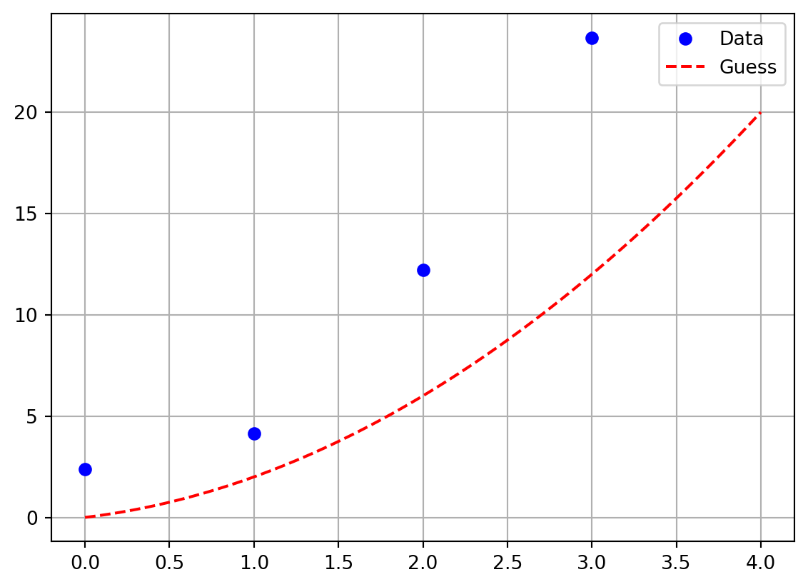
Exercise 5.19 Now let us be a bit more systematic about things from the previous exercise. Let us say that you have a pretty good guess that \(b \approx 2\) and \(c \approx 0.7\). We need to get a good estimate for \(a\).
Pick an arbitrary starting value for \(a\) then for each of the four points find the error between the predicted \(y\) value and the actual \(y\) value. These errors are called the residuals.
Square all four of your errors and add them up. (Pause, ponder, and discuss: why are we squaring the errors before we sum them?)
Now change your value of \(a\) to several different values and record the sum of the square errors for each of your values of \(a\).
Make a plot with the value of \(a\) on the horizontal axis and the value of the sum of the square errors on the vertical axis. Use your plot to defend the optimal choice for \(a\).
Clearly the above is calling for some Python code to automate this exploration. Write a loop that tries many values of \(a\) in very small increments and calculates the sum of the squared errors. The following partial Python code should help you get started. In the resulting plot you should see a clear local minimum. What does that minimum tell you about solving this problem?
import numpy as np
import matplotlib.pyplot as plt
xdata = np.array([0, 1, 2, 3])
ydata = np.array([2.37, 4.14, 12.22, 23.68])
b = 2
c = 0.75
A = # give a numpy array of values for a
SumSqRes = [] # this is storage for the sum of the sq. residuals
for a in A:
  guess = a*xdata**2 + b*xdata + c
  residuals = # write code to calculate the residuals
  SumSqRes.append( ??? ) # calculate the sum of the squ. residuals
plt.plot(A,SumSqRes,'r*')
plt.grid()
plt.xlabel('Value of a')
plt.ylabel('Sum of squared residuals')
plt.show()
Now let us formalize the process that we have described in the previous exercises.
Let \[\begin{equation} S = \{ (x_0, y_0), \, (x_1, y_1), \, \ldots, \, (x_n, y_n) \} \end{equation}\] be a set of \(n+1\) ordered pairs in \(\mathbb{R}^2\). If we guess that a function \(f(x)\) is a best choice to fit the data and if \(f(x)\) depends on parameters \(a_0, a_n, \ldots, a_n\) then
Pick initial values for the parameters \(a_0, a_1, \ldots, a_n\) so that the function \(f(x)\) looks like it is close to the data (this is strictly a visual step …take care that it may take some playing around to guess the initial values of the parameters)
Calculate the square error between the data point and the prediction from the function \(f(x)\) \[\begin{equation} \text{error for the point $x_i$: } e_i = \left( y_i - f(x_i) \right)^2. \end{equation}\] Note that squaring the error has the advantages of removing the sign, accentuating errors larger than 1, and decreasing errors that are less than 1.
As a measure of the total error between the function and the data, sum the squared errors \[\begin{equation} \text{sum of square errors } = \sum_{i=1}^n \left( y_i - f(x_i) \right)^2. \end{equation}\] (Take note that if there were a continuum of points instead of a discrete set then we would integrate the square errors instead of taking a sum.)
Change the parameters \(a_0, a_1, \ldots\) so as to minimize the sum of the square errors.
Exercise 5.20 The last step above is a bit vague. That was purposeful since there are many techniques that could be used to minimize the sum of the square errors. However, if we just think about the sum of the squared residuals as a function then we can apply scipy.optimize.minimize() to that function in order to return the values of the parameters that best minimize the sum of the squared residuals. The following blocks of Python code implement the idea in a very streamlined way. Go through the code and comment each line to describe exactly what it does.
import numpy as np
import matplotlib.pyplot as plt
from scipy.optimize import minimize
xdata = np.array([0, 1, 2, 3])
ydata = np.array([2.37, 4.14, 12.22, 23.68])

def SSRes(parameters):
  # In the next line of code we want to build our
  # quadratic approximation y = ax^2 + bx + c
  # We are sending in a list of parameters so
  # a = parameters[0], b = parameters[1], and c = parameters[2]
  yapprox = parameters[0]*xdata**2 + \
            parameters[1]*xdata + \
            parameters[2]
  residuals = np.abs(ydata-yapprox)
  return np.sum(residuals**2)


BestParameters = minimize(SSRes,[1,1,1])
print("The best values of a, b, and c are: \n",BestParameters.x)
# If you want to print the diagnositc then use the line below:
# print("The minimization diagnostics are: \n",BestParameters)plt.plot(xdata,ydata,'bo')
x = np.linspace(0,4,100)
y = BestParameters.x[0]*x**2 + \
BestParameters.x[1]*x + \
BestParameters.x[2]
plt.plot(x,y,'r--')
plt.grid()
plt.xlabel('x')
plt.ylabel('y')
plt.title('Best Fit Quadratic')
plt.show()Exercise 5.21 Now I’ll let you in on a little secret: the data that you have fitted the quadratic function to above was not real data. I created it with the following script.
import numpy as np
# Set a seed for the random number generator
np.random.seed(1)
# Use a quadratic function to generate some fake data
a, b, c = 2, 2, 0.75
f = lambda x: a*x**2 + b*x + c
# Choose 4 equally-spaced x-values
xdata = np.linspace(0,3,4)
# Add normally distributed errors to the y values
ydata = f(xdata) + np.random.normal(0,1,4)
# round to two digits
ydata = np.around(ydata, 2)
print(xdata)
print(ydata)
[0. 1. 2. 3.]
[ 2.37 4.14 12.22 23.68]Such fake data that is generated from a know function with known distribution of the error is referred to as “synthetic data” and is very useful for testing parameter fitting methods.
You will notice that the parameters that we estimated with the Least Squares method are not at all the same as the parameters that I used to generate the data. This is because we had only 4 noise data points to estimate 3 parameters.
Adjust the above script so that it generates 100 \(x\) values between 0 and 3 and corresponding noise \(y\) values. Then try to estimate the parameters of the quadratic function that generated the data. Does the estimate get closer to the original parameter values?
Exercise 5.22 In your group choose a function with a small number of parameters and choose parameter values and then evaluate 50 points on that function. Add a small bit of error into the \(y\)-values of your points. Give your 50 points to another group together with the definition of the function. Upon receiving your new points:
Plot your points.
Make a guess about the basic form of the function that might best fit the data.
Modify the code from above to find the best collection of parameters to minimize the sum of the squares of the residuals between the function and the data.
Plot the data along with your best fit function.
Go back to the group who gave you your points and check your work.
Using the method of least squares to fit a function to data is not always the right thing to do. It is appropriate if the measurement error in the data is normally distributed with the same variance for all data points and if the errors are independent of each other. If the errors are not normally distributed or if they are not independent of each other then the method of least squares is not appropriate. In such cases a more sophisticated method of fitting the data is needed. This is a large and active area of research and we will not go into more detail here.
Exercise 5.23 Explain in clear language how the Golden Section Search method works.
Exercise 5.24 Explain in clear language how the Gradient Descent method works.
Exercise 5.25 Explain in clear language how you use the method of Least Squares to fit a function to data.
Exercise 5.26 For each of the following functions write code to numerically approximate the local maximum or minimum that is closest to \(x=0\). You may want to start with a plot of the function just to get a feel for where the local extreme value(s) might be.
\(\displaystyle f(x) = \frac{x}{1+x^4} + \sin(x)\)
\(\displaystyle g(x) = \left(x-1\right)^3\cdot\left(x-2\right)^2+e^{-0.5\cdot x}\)
Exercise 5.27 (This exercise is modified from (Meerschaert 2013))
A pig weighing 200 pounds gains 5 pounds per day and costs 45 cents a day to keep. The market price for pigs is 65 cents per pound, but is falling 1 cent per day. When should the pig be sold to maximize the profit?
Write the expression for the profit \(P(t)\) as a function of time \(t\) and maximize this analytically (by hand). Then solve the problem with all three methods outlined in Section 5.1.
Exercise 5.28 (This exercise is modified from (Meerschaert 2013))
Reconsider the pig Exercise 5.27 but now suppose that the weight of the pig after \(t\) days is \[\begin{equation}
w = \frac{800}{1+3e^{-t/30}} \text{ pounds}.
\end{equation}\] When should the pig be sold and how much profit do you make on the pig when you sell it? Write this situation as a single variable mathematical model. You should notice that the algebra and calculus for solving this problem is no longer really a desirable way to go. Use an appropriate numerical technique to solve this problem.
Exercise 5.29 Go back to your old Calculus textbook or homework and find your favourite optimization problem. State the problem, create the mathematical model, and use any of the numerical optimization techniques in this chapter to get an approximate solution to the problem.
Exercise 5.30 In the code below you can download several sets of noisy data from measurements of elementary single variable functions.
Make a hypothesis about which type of function would best model the data. Be sure to choose the most general (parametrized) form of your function.
Use appropriate tools to find the parameters for the function that best fits the data. Report you sum of square residuals for each function.
The functions that you propose must be continuous functions.
import numpy as np
import pandas as pd
URL = 'https://github.com/gustavdelius/NumericalAnalysis2024/raw/main/data/Optimization/'
datasetA = np.array( pd.read_csv(URL+'Exercise3_datafit5.csv') )
datasetB = np.array( pd.read_csv(URL+'Exercise3_datafit6.csv') )
datasetC = np.array( pd.read_csv(URL+'Exercise3_datafit7.csv') )
datasetD = np.array( pd.read_csv(URL+'Exercise3_datafit8.csv') )
datasetE = np.array( pd.read_csv(URL+'Exercise3_datafit9.csv') )
datasetF = np.array( pd.read_csv(URL+'Exercise3_datafit10.csv') )
datasetG = np.array( pd.read_csv(URL+'Exercise3_datafit11.csv') )
datasetH = np.array( pd.read_csv(URL+'Exercise3_datafit12.csv') )
# Exercise3_datafit5.csv - Exercise3_datafit12.csv
Exercise 5.31 (The Goat Problem) This is a classic problem in recreational mathematics that has a great approximate solution where we can leverage some of our numerical analysis skills. Grab a pencil and a piece of paper so we can draw a picture.
Draw a coordinate plane
Draw a circle with radius 1 unit centred at the point \((0,1)\). This circle will obviously be tangent to the \(x\) axis.
Draw a circle with radius \(r\) centred at the point \((0,0)\). We will take \(0 < r < 2\) so there are two intersections of the two circles.
Label the left-hand intersection of the two circles as point \(A\). (Point \(A\) should be in the second quadrant of your coordinate plane.)
Label the right-hand intersection of the circles as point \(B\). (Point \(B\) should be in the first quadrant of your coordinate plane.)
Label the point \((0,0)\) as the point \(P\).
A rancher has built a circular fence of radius 1 unit centred at the point \((0,1)\) for his goat to graze. He tethers his goat at point \(P\) on the far south end of the circular fence. He wants to make the length of the goat’s chain, \(r\), just long enough so that it can graze half of the area of the fenced region. How long should he make the chain?
Hints:
It would be helpful to write equations for both circles. Then you can use the equations to find the coordinates of the intersection points \(A\) and \(B\).
You can either solve for the intersection points algebraically or you can use a numerical root finding technique to find the intersection points.
In any case, the intersection points will (obviously) depend on the value of \(r\)
Set up an integral to find the area grazed by the goat.
Write code to narrow down on the best value of \(r\) where the integral evaluates to half the area of the fenced region.
In this section we propose several ideas for projects related to numerical optimisation. These projects are meant to be open ended, to encourage creative mathematics, to push your coding skills, and to require you to write and communicate your mathematics.
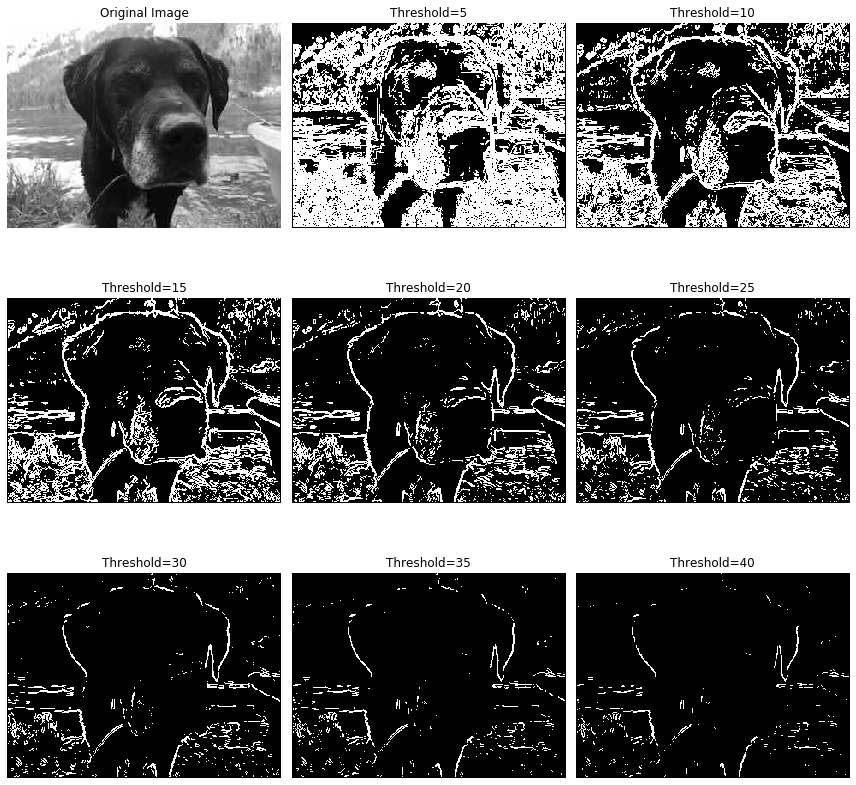
Edge detection is the process of finding the boundaries or edges of objects in an image. There are many approaches to performing edge detection, but one method that is quite robust is to use the gradient vector in the following way:
First convert the image to gray scale.
Then think of the gray scale image as a plot of a multivariable function \(G(x,y)\) where the ordered pair \((x,y)\) is the pixel location and the output \(G(x,y)\) is the value of the gray scale at that point.
At each pixel calculate the gradient of the function \(G(x,y)\) numerically.
If the magnitude of the gradient is larger than some threshold then the function \(G(x,y)\) is steep at that location and it is possible that there is an edge (a transition from one part of the image to a different part) at that point. Hence, if \(\|\nabla G(x,y)\| > \delta\) for some threshold \(\delta\) then we can mark the point \((x,y)\) as an edge point.
Your Tasks:
Choose several images on which to do edge detection. You should take your own images, but if you choose not to be sure that you cite the source(s) of your images.
Write Python code that performs edge detection as described above on the image. In the end you should produce side-by-side plots of the original picture and the image showing only the edges. To calculate the gradient use a centred difference scheme for the first derivatives \[\begin{equation}
f'(x) \approx \frac{f(x+h)-f(x-h)}{2h}.
\end{equation}\] In an image we can take \(h=1\) (why?), and since the gradient is two dimensional we get \[\begin{equation}
\nabla G(x,y) \approx \left< \frac{G(x+1,y)-G(x-1,y)}{2} \, , \, \frac{G(x,y+1)-G(x,y-1)}{2} \right>.
\end{equation}\] Figure 5.6 depicts what this looks like when we zoom in to a pixel and its immediate neighbours. The pixel labelled G[i,j] is the pixel at which we want to evaluate the gradient, and the surrounding pixels are labelled by their indices relative to [i,j].
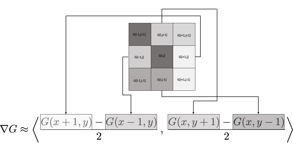
[i,j]. Also notice that we did not reach out any further than a single pixel. Your job now is to build several other approaches to calculating the gradient vector, implement them to perform edge detection, and show the resulting images. For each method you need to give the full mathematical details for how you calculated the gradient as well as give a list of pros and cons for using the new numerical gradient for edge detection based on what you see in your images. As an example, you could use a centred difference scheme that looks two pixels away instead of at the immediate neighbouring pixels \[\begin{equation}
f'(x) \approx \frac{??? f(x-2) + ??? f(x+2)}{???}.
\end{equation}\] Of course you would need to determine the coefficients in this approximation scheme.The following code will allow you to read an image into Python as an np.array().
import numpy as np
import matplotlib.pyplot as plt
from matplotlib import image
I = np.array(image.plt.imread('ImageName.jpg'))
plt.imshow(I)
plt.axis("off")
plt.show()
You should notice that the image, I, is a three dimensional array. The three layers are the red, green, and blue channels of the image. To flatten the image to gray scale you can apply the rule \[\begin{equation}
\text{grayscale value} = 0.3 \text{Red} + 0.59 \text{Green} + 0.11 \text{Blue}.
\end{equation}\] The output should be a 2 dimensional numpy array which you can show with the following Python code.
plt.imshow(G, cmap='gray') # "cmap" stands for "color map"
plt.axis("off")
plt.show()
Figure 5.7 shows the result of different threshold values applied to the simplest numerical gradient computations. The image was taken by the author.