2 Approximations

We think in generalities, but we live in details.
–Alfred North Whitehead

Have you ever wondered how computers, which operate in a realm of zeros and ones, manage to perform mathematical calculations with real numbers? The secret lies in approximation.

In this chapter we will investigate the foundations that allow a computer to do mathematical calculations at all. How can it store real numbers? How can it calculate the values of mathematical functions? We will understand that the computer can do these things only approximately and will thus always make errors. Numerical Analysis is all about keeping these errors as small as possible while still being able to do efficient calculations.

We will meet the two kinds of errors that a computer makes: rounding errors and truncation errors. Rounding errors arise from the way the computer needs to approximate real numbers by binary floating point numbers, which are the numbers it know how to add, subtract, multiply and divide. Truncation errors arise from the way the computer needs to reduce all calculations to a finite number of these four basic arithmetic operations. We see that in this chapter when we discuss how computers approximate functions by power series and then have to truncate these at some finite order.

2.1 Binary Numbers

Exercise 2.1 By hand (no computers!) compute the first 50 terms of this sequence with the initial condition $x_0 = 1/10$.

\[\begin{equation} x_{n+1} = \left\{ \begin{array}{ll} 2x_n, & x_n \in [0,\frac{1}{2}] \\ 2x_n - 1, & x_n \in (\frac{1}{2},1] \end{array} \right. \end{equation}\]

Exercise 2.2 Now use a spreadsheet and to do the computations. Do you get the same answers?

Exercise 2.3 Finally, solve this problem with Python. Some starter code is given to you below.

x = 1.0/10
for n in range(50):
    if x<= 0.5:
        # put the correct assignment here
    else:
        # put the correct assigment here
    print(x)

Exercise 2.4 It seems like the computer has failed you! What do you think happened on the computer and why did it give you a different answer? What, do you suppose, is the cautionary tale hiding behind the scenes with this problem?

Exercise 2.5 Now what happens with this problem when you start with $x_0 = 1/8$? Why does this new initial condition work better?

A computer circuit knows two states: on and off. As such, anything saved in computer memory is stored using base-2 numbers. This is called a binary number system. To fully understand a binary number system it is worth while to pause and reflect on our base-10 number system for a few moments.

What do the digits in the number “735” really mean? The position of each digit tells us something particular about the magnitude of the overall number. The number 735 can be represented as a sum of powers of 10 as

\[\begin{equation} 735 = 700 + 30 + 5 = 7 \times 10^2 + 3 \times 10^1 + 5 \times 10^0 \end{equation}\]

and we can read this number as 7 hundreds, 3 tens, and 5 ones. As you can see, in a “positional number system” such as our base-10 system, the position of the number indicates the power of the base, and the value of the digit itself tells you the multiplier of that power. This is contrary to number systems like Roman Numerals where the symbols themselves give us the number, and meaning of the position is somewhat flexible. The number “48,329” can therefore be interpreted as

\[\begin{equation} \begin{split} 48,329 &= 40,000 + 8,000 + 300 + 20 + 9 \\ &= 4 \times 10^4 + 8 \times 10^3 + 3 \times 10^2 + 2 \times 10^1 + 9 \times 10^0, \end{split} \end{equation}\]

four ten thousands, eight thousands, three hundreds, two tens, and nine ones.

Now let us switch to the number system used by computers: the binary number system. In a binary number system the base is 2 so the only allowable digits are 0 and 1 (just like in base-10 the allowable digits were 0 through 9). In binary (base-2), the number “101,101” can be interpreted as

\[\begin{equation} 101,101_2 = 1 \times 2^5 + 0 \times 2^4 + 1 \times 2^3 + 1 \times 2^2 + 0 \times 2^1 + 1 \times 2^0 \end{equation}\]

(where the subscript “2” indicates the base to the reader). If we put this back into base 10, so that we can read it more comfortably, we get

\[101,101_2 = 32 + 0 + 8 + 4 + 0 + 1 = 45_{10}.\]

The reader should take note that the commas in the numbers are only to allow for greater readability – we can easily see groups of three digits and mentally keep track of what we are reading.

Exercise 2.6 Express the following binary numbers in base-10.

$111_2$
$10,101_2$
$1,111,111,111_2$

Exercise 2.7 Explain the joke: There are 10 types of people. Those who understand binary and those who do not.

Exercise 2.8 Discussion: With your group, discuss how you would convert a base-10 number into its binary representation. Once you have a proposed method put it into action on the number $237_{10}$ to show that the base-2 expression is $11,101,101_2$.

Exercise 2.9 Convert the following numbers from base 10 to base 2 or visa versa.

Write $12_{10}$ in binary
Write $11_{10}$ in binary
Write $23_{10}$ in binary
Write $11_2$ in base $10$
What is $100101_2$ in base $10$?

Exercise 2.10 Now that you have converted several base-10 numbers to base-2, summarize an efficient technique to do the conversion.

Example 2.1 Convert the number $137$ from base $10$ to base $2$.

Solution. One way to do the conversion is to first look for the largest power of $2$ less than or equal to your number. In this case, $128=2^7$ is the largest power of $2$ that is less than $137$. Then looking at the remainder, $9$, look for the largest power of $2$ that is less than this remainder. Repeat until you have the number.

\[\begin{aligned} 137_{10} &= 128 + 8 + 1 \\ &= 2^7 + 2^3 + 2^0 \\ &= 1 \times 2^7 + 0 \times 2^6 + 0 \times 2^5 + 0 \times 2^4 + 1 \times 2^3 + 0 \times 2^2 + 0 \times 2^1 + 1 \times 2^0 \\ &= 10001001_2 \end{aligned}\]

Next we will work with fractions and decimals.

Example 2.2 Let us take the base $10$ number $5.341_{10}$ and expand it out to get

\[5.341_{10} = 5 + \frac{3}{10} + \frac{4}{100} + \frac{1}{1000} = 5 \times 10^0 + 3 \times 10^{-1} + 4 \times 10^{-2} + 1 \times 10^{-3}.\]

The position to the right of the decimal point is the negative power of 10 for the given position.

We can do a similar thing with binary decimals.

Exercise 2.11 The base-2 number $1,101.01_2$ can be expanded in powers of $2$. Fill in the question marks below and observe the pattern in the powers.

\[1,101.01_2 = ? \times 2^3 + 1 \times 2^2 + 0 \times 2^1 + ? \times 2^0 + 0 \times 2^{?} + 1 \times 2^{-2}.\]

Example 2.3 Convert $11.01011_2$ to base $10$.
Solution:

\[\begin{aligned} 11.01011_2 &= 2 + 1 + \frac{0}{2} + \frac{1}{4} + \frac{0}{8} + \frac{1}{16} + \frac{1}{32} \\ &= 1 \times 2^1 + 1 \times 2^0 + 0 \times 2^{-1} + 1 \times 2^{-2} + 0 \times 2^{-3} + 1 \times 2^{-4} + 1 \times 2^{-5}\\ &= 3.34375_{10}. \end{aligned}\]

Exercise 2.12 Repeating digits in binary numbers are rather intriguing. The number $0.\overline{0111} = 0.01110111011101110111\ldots$ surely also has a decimal representation. I will get you started:

\[\begin{aligned} 0.0_2 &= 0 \times 2^0 + 0 \times 2^{-1} = 0.0_{10} \\ 0.01_2 &= 0.0_{10} + 1 \times 2^{-2} = 0.25_{10} \\ 0.011_2 &= 0.25_{10} + 1 \times 2^{-3} = 0.25_{10} + 0.125_{10} = 0.375_{10} \\ 0.0111_2 &= 0.375_{10} + 1 \times 2^{-4} = 0.4375_{10} \\ 0.01110_2 &= 0.4375_{10} + 0 \times 2^{-5} = 0.4375_{10} \\ 0.011101_2 &= 0.4375_{10} + 1 \times 2^{-6} = 0.453125_{10} \\ \vdots & \qquad \qquad \vdots \qquad \qquad \qquad \vdots \end{aligned}\]

We want to know what this series converges to in base 10. Work with your partners to approximate the base-10 number.

Exercise 2.13 Convert the following numbers from base 10 to binary.

What is $1/2$ in binary?
What is $1/8$ in binary?
What is $4.125$ in binary?
What is $0.15625$ in binary?

Exercise 2.14 Convert the base $10$ decimal $0.635$ to binary using the following steps.

Multiply $0.635$ by $2$. The whole number part of the result is the first binary digit to the right of the decimal point.
Take the result of the previous multiplication and ignore the digit to the left of the decimal point. Multiply the remaining decimal by $2$. The whole number part is the second binary decimal digit.
Repeat the previous step until you have nothing left, until a repeating pattern has revealed itself, or until your precision is close enough.

Explain why each step gives the binary digit that it does.

Exercise 2.15 Based on your previous problem write an algorithm that will convert base-10 decimals (less than 1) to binary.

Exercise 2.16 Convert the base $10$ fraction $1/10$ into binary. Use your solution to fully describe what went wrong in the Exercise 2.1.

2.2 Floating Point Numbers

Everything stored in the memory of a computer is a number, but how does a computer actually store a number. More specifically, since computers only have finite memory we would really like to know the full range of numbers that are possible to store in a computer. Clearly, given the uncountable nature of the real numbers, there will be gaps between the numbers that can be stored. We would like to know what gaps in our number system to expect when using a computer to store and do computations on numbers.

Exercise 2.17 Let us start the discussion with a very concrete example. Consider the number $x = -123.15625$ (in base 10). As we have seen this number can be converted into binary. Indeed

\[x = -123.15625_{10} = -1111011.00101_2\]

(you should check this).

If a computer needs to store this number then first they put in the binary version of scientific notation. In this case we write

\[x = -1. \underline{\hspace{1in}} \times 2^{\underline{\hspace{0.25in}}}\]
Based on the fact that every binary number, other than 0, can be written in this way, what three things do you suppose a computer needs to store for any given number?
Using your answer to part (b), what would a computer need to store for the binary number $x=10001001.1100110011_2$?

Definition 2.1 For any base-2 number $x$ we can write

\[x = (-1)^{s} \times (1+ m) \times 2^E\]

where $s \in \{0,1\}$ and $m$ is a binary number such that $0 \le m < 1$.

The number $m$ is called the mantissa or the significand, $s$ is known as the sign bit, and $E$ is known as the exponent.

Example 2.4 What are the mantissa, sign bit, and exponent for the numbers $7_{10}, -7_{10}$, and $(0.1)_{10}$?
Solution:

For the number $7_{10}=111_2 = 1.11 \times 2^2$ we have $s=0, m=0.11$ and $E=2$.
For the number $-7_{10}=111_2 = -1.11 \times 2^2$ we have $s=1, m=0.11$ and $E=2$.
For the number $\frac{1}{10} = 0.000110011001100\cdots = 1.100110011 \times 2^{-4}$ we have $s=0, m=0.100110011\cdots$, and $E = -4$.

In the last part of the previous example we saw that the number $(0.1)_{10}$ is actually a repeating decimal in base-2. This means that in order to completely represent the number $(0.1)_{10}$ in base-2 we need infinitely many decimal places. Obviously that cannot happen since we are dealing with computers with finite memory. Over the course of the past several decades there have been many systems developed to properly store numbers. The IEEE standard that we now use is the accumulated effort of many computer scientists, much trial and error, and deep scientific research. We now have three standard precisions for storing numbers on a computer: single, double, and extended precision. The double precision standard is what most of our modern computers use.

Definition 2.2 There are two common precisions for storing numbers in a computer.

A single-precision number consists of 32 bits, with 1 bit for the sign, 8 for the exponent, and 23 for the significand.
A double-precision number consists of 64 bits with 1 bit for the sign, 11 for the exponent, and 52 for the significand.

Definition 2.3 (Machine precision) Machine precision is the gap between the number 1 and the next larger floating point number. Often it is represented by the symbol $\epsilon$. To clarify, the number 1 can always be stored in a computer system exactly and if $\epsilon$ is machine precision for that computer then $1+\epsilon$ is the next largest number that can be stored with that machine.

For all practical purposes the computer cannot tell the difference between two numbers if the difference is smaller than machine precision. This is of the utmost important when you want to check that something is “zero” since a computer just cannot know the difference between $0$ and $\epsilon$.

Exercise 2.18 To make all of these ideas concrete let us play with a small computer system where each number is stored in the following format:

\[s \, E \, b_1 \, b_2 \, b_3\]

The first entry is a bit for the sign ($0=+$ and $1=-$). The second entry, $E$ is for the exponent, and we will assume in this example that the exponent can be 0, 1, or $-1$. The three bits on the right represent the significand of the number. Hence, every number in this number system takes the form

\[(-1)^s \times (1+ 0.b_1b_2b_3) \times 2^{E}\]

What is the smallest positive number that can be represented in this form?
What is the largest positive number that can be represented in this form?
What is the machine precision in this number system?
What would change if we allowed $E \in \{-2,-1,0,1,2\}$?

Exercise 2.19 What are the largest and smallest numbers that can be stored in single and double precision?

Exercise 2.20 What is machine precision for the single and double precision standard?

Exercise 2.21 What is the gap between $2^n$ and the next largest number that can be stored in double precision?

Much more can be said about floating point numbers such as how we store infinity, how we store NaN, and how we store 0. The Wikipedia page for floating point arithmetic might be of interest for the curious reader. It is beyond the scope of this module to go into all of those details here. Instead, the biggest takeaway points from this section and the previous are:

All numbers in a computer are stored with finite precision.
Nice numbers like 0.1 are sometimes not machine representable in binary.
Machine precision is the gap between 1 and the next largest number that can be stored.
The gap between one number and the next grows in proportion to the number.

2.3 Loss of significant digits

As we have discussed, when representing real numbers by floating point numbers in the computer, rounding errors will usually occur. However each individual rounding error is only a tiny fraction of the actual number, so should not really matter. However, calculations usually involve a number of steps, and if we are not careful then the rounding errors can get magnified if we perform the steps in an unfortunate way. The following exercises will illustrate this.

Example 2.5 Consider the expression \[ (10^{10} + 0.123456789) - 10^{10}. \] Mathematically the two terms of $10^{10}$ simply cancel out leaving just $0.123456789$. However, let us evaluate this in Python:

10**10 + 0.123456789 - 10**10

0.12345695495605469

Only the first six digits after the decimal point were preserved, the other digits were replaced by something seemingly random. The reason should be clear. The computer makes a rounding error when it tries to store the $10000000000.123456789$. This is known as the loss of significant digits. It occurs whenever you subtract two almost equal numbers from each other.

Exercise 2.22 Consider the trigonometric idenity \[ 2\sin^2(x/2) = 1 - \cos(x). \] It gives us two different methods to calculate the same quantity. Ask Python to evaluate both sides of the identity. If you want to calculate $1 - \cos(x)$ with the highest precision, which expression would you use? Discuss.

Exercise 2.23 You know how fo find the solutions to the quadratic equation \[ a x^2+bx+c=0. \] You know the quadratic formula. For the larger of the two solutions the formula is \[ x = \frac{-b+\sqrt{b^2-4ac}}. \] Let’s assume that the parameters are given as \[ a = 1,~~~b = 1000000, ~~~ c = 1.\] Use the quadratic formula to find the larger of the two solutions, by coding the formula up in Python. You should get a solution slightly larger than 1. Then check whether your value for $x$ really does solve the quadratic equation by evaluating $ax^2+bx+c$ with your value of $x$. You will notice that it does not work. Discuss the cause of the error.

Now rearrange the quadratic formula for the larger solution by multiplying both the numerator and denominator by $-b-\sqrt{b^2-4ac}$ and then simplify by multiplying out the resulting numerator. This should give you the alternative formula \[ x = \frac{2c}{-b-\sqrt{b^2-4ac}}. \] Can you see why this expression will work better for the given parameter values? Again evaluate $x$ with Python and then check it by substituting into the quadratic expression. What do you find?

These exercises should suffice to make you sensitive to the issue of loss of significant figures.

2.4 Approximating Functions

How does a computer understand a function like $f(x) = e^x$ or $f(x) = \sin(x)$ or $f(x) = \log(x)$? What happens under the hood, so to speak, when you ask a computer to do a computation with one of these functions? A computer is darn good at arithmetic, but working with transcendental functions like these, or really any other sufficiently complicated functions for that matter, is not something that comes naturally to a computer. What is actually happening under the hood is that the computer only approximates the functions.

Exercise 2.24 In this problem we are going to make a bit of a wish list for all of the things that a computer will do when approximating a function. We are going to complete the following sentence:
If we are going to approximate a smooth function $f(x)$ near the point $x=x_0$ with a simpler function $g(x)$ then …

(I will get us started with the first two things that seems natural to wish for. The rest of the wish list is for you to complete.)

the functions $f(x)$ and $g(x)$ should agree at $x=x_0$. In other words, $f(x_0) = g(x_0)$
the function $g(x)$ should only involve addition, subtraction, multiplication, division, and integer exponents since computer are very good at those sorts of operations.
if $f(x)$ is increasing / decreasing near $x=x_0$ then $g(x)$ …
if $f(x)$ is concave up / down near $x=x_0$ then $g(x)$…
if we zoom into plots of the functions $f(x)$ and $g(x)$ near $x=x_0$ then …
… is there anything else that you would add?

Exercise 2.25 Discuss: Could a polynomial function with a high enough degree satisfy everything in the wish list from the previous problem? Explain your reasoning.

Exercise 2.26 Let us put some parts of the wish list into action. If $f(x)$ is a differentiable function at $x=x_0$ and if $g(x) = A + B (x-x_0) + C (x-x_0)^2 + D (x-x_0)^3$ then

What is the value of $A$ such that $f(x_0) = g(x_0)$? (Hint: substitute $x=x_0$ into the $g(x)$ function)
What is the value of $B$ such that $f'(x_0) = g'(x_0)$? (Hint: Start by taking the derivative of $g(x)$)
What is the value of $C$ such that $f''(x_0) = g''(x_0)$?
What is the value of $D$ such that $f'''(x_0) = g'''(x_0)$?

Exercise 2.27 Let $f(x) = e^x$. Put the answers to the previous question into action and build a cubic polynomial that approximates $f(x) = e^x$ near $x_0=0$.

In the previous 4 exercises you have built up some basic intuition for what we would want out of a mathematical operation that might build an approximation of a complicated function. What we have built is actually a way to get better and better approximations for functions out to pretty much any arbitrary accuracy that we like so long as we are near some anchor point (which we called $x_0$ in the previous exercises).

In the next several problems you will unpack the approximations of $f(x) = e^x$ a bit more carefully and we will wrap the whole discussion with a little bit of formal mathematical language. Then we will examine other functions like sine, cosine, logarithms, etc. One of the points of this whole discussion is to give you a little glimpse as to what is happening behind the scenes in scientific programming languages when you do computations with these functions. A bigger point is to start getting a feel for how we might go in reverse and approximate an unknown function out of much simpler parts. This last goal is one of the big takeaways from numerical analysis: we can mathematically model highly complicated functions out of fairly simple pieces.

Exercise 2.28 What is Euler’s number $e$? You likely remember using this number often in Calculus and Differential Equations. Do you know the decimal approximation for this number? Moreover, is there a way that we could approximate something like $\sqrt{e} = e^{0.5}$ or $e^{-1}$ without actually having access to the full decimal expansion?

For all of the questions below let us work with the function $f(x) = e^x$.

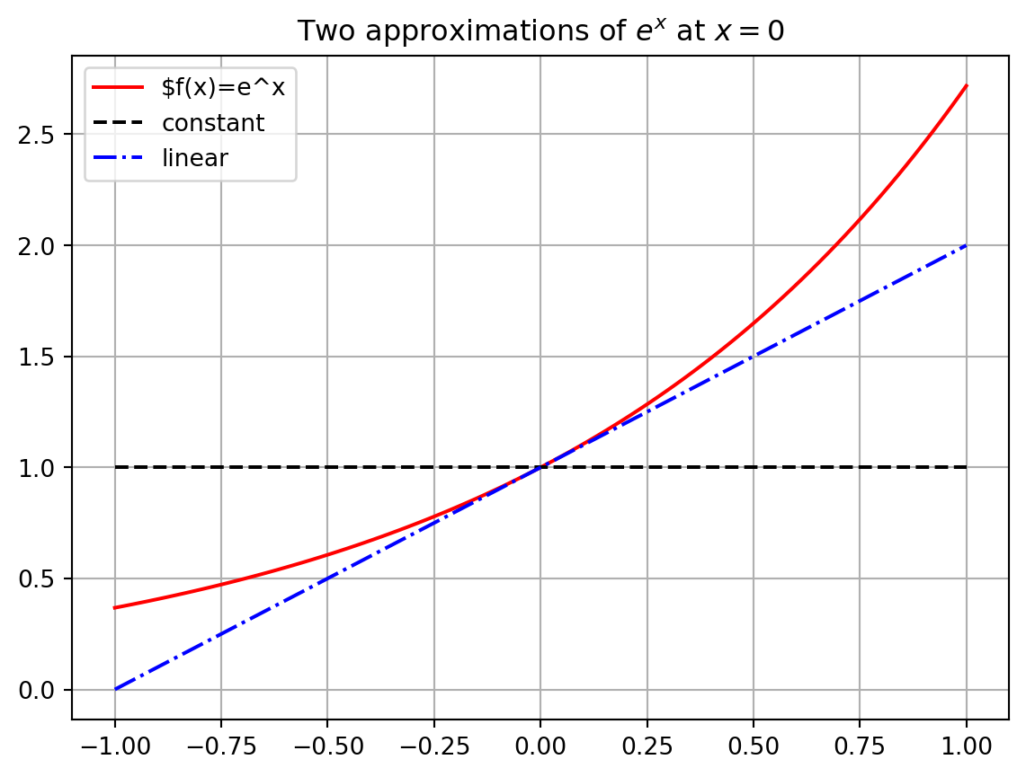
The function $g(x) = 1$ matches $f(x) = e^x$ exactly at the point $x=0$ since $f(0) = e^0 = 1$. Furthermore if $x$ is very very close to $0$ then the functions $f(x)$ and $g(x)$ are really close to each other. Hence we could say that $g(x) = 1$ is an approximation of the function $f(x) = e^x$ for values of $x$ very very close to $x=0$. Admittedly, though, it is probably pretty clear that this is a horrible approximation for any $x$ just a little bit away from $x=0$.
Let us get a better approximation. What if we insist that our approximation $g(x)$ matches $f(x) = e^x$ exactly at $x=0$ and ALSO has exactly the same first derivative as $f(x)$ at $x=0$.
1. What is the first derivative of $f(x)$?
2. What is $f'(0)$?
3. Use the point-slope form of a line to write the equation of the function $g(x)$ that goes through the point $(0,f(0))$ and has slope $f'(0)$. Recall from algebra that the point-slope form of a line is $y = f(x_0) + m(x-x_0).$ In this case we are taking $x_0 = 0$ so we are using the formula $g(x) = f(0) + f'(0) (x-0)$ to get the equation of the line.
Write Python code to build a plot like Figure 2.1. This plot shows $f(x) = e^x$, our first approximation $g(x) = 1$ and our second approximation $g(x) = 1+x$. You may want to refer back to Exercise 1.22 in the Python chapter.

Figure 2.1: The first two polynomial approximations of the exponential function.

Exercise 2.29 Let us extend the idea from the previous problem to much better approximations of the function $f(x) = e^x$.

Let us build a function $g(x)$ that matches $f(x)$ exactly at $x=0$, has exactly the same first derivative as $f(x)$ at $x=0$, AND has exactly the same second derivative as $f(x)$ at $x=0$. To do this we will use a quadratic function. For a quadratic approximation of a function we just take a slight extension to the point-slope form of a line and use the equation \[\begin{equation} y = f(x_0) + f'(x_0) (x-x_0) + \frac{f''(x_0)}{2} (x-x_0)^2. \end{equation}\] In this case we are using $x_0 = 0$ so the quadratic approximation function looks like \[\begin{equation} y = f(0) + f'(0) x + \frac{f''(0)}{2} x^2. \end{equation}\]
1. Find the quadratic approximation for $f(x) = e^x$.
2. How do you know that this function matches $f(x)$ is all of the ways described above at $x=0$?
3. Add your new function to the plot you created in the previous problem.
Let us keep going!! Next we will do a cubic approximation. A cubic approximation takes the form \[\begin{equation} y = f(x_0) + f'(0) (x-x_0) + \frac{f''(0)}{2}(x-x_0)^2 + \frac{f'''(0)}{3!}(x-x_0)^3 \end{equation}\]
1. Find the cubic approximation for $f(x) = e^x$.
2. How do we know that this function matches the first, second, and third derivatives of $f(x)$ at $x=0$?
3. Add your function to the plot.
4. Pause and think: What’s the deal with the $3!$ on the cubic term?
Your turn: Build the next several approximations of $f(x) = e^x$ at $x=0$. Add these plots to the plot that we have been building all along.

Exercise 2.30 Use the functions that you have built to approximate $\frac{1}{e} = e^{-1}$. Check the accuracy of your answer using np.exp(-1) in Python.

What we have been exploring so far in this section is the Taylor Series of a function.

Definition 2.4 (Taylor Series) If $f(x)$ is an infinitely differentiable function at the point $x_0$ then \[\begin{equation} f(x) = f(x_0) + f'(x_0)(x-x_0) + \frac{f''(x_0)}{2}(x-x_0)^2 + \cdots \frac{f^{(n)}(x_0)}{n!}(x-x_0)^n + \cdots \end{equation}\] for any reasonably small interval around $x_0$. The infinite polynomial expansion is called the Taylor Series of the function $f(x)$. Taylor Series are named for the mathematician Brook Taylor.

The Taylor Series of a function is often written with summation notation as \[\begin{equation} f(x) = \sum_{k=0}^\infty \frac{f^{(k)}(x_0)}{k!} (x-x_0)^k. \end{equation}\] Do not let the notation scare you. In a Taylor Series you are just saying: give me a function that

matches $f(x)$ at $x=x_0$ exactly,
matches $f'(x)$ at $x=x_0$ exactly,
matches $f''(x)$ at $x=x_0$ exactly,
matches $f'''(x)$ at $x=x_0$ exactly,
etc.

(Take a moment and make sure that the summation notation makes sense to you.)

Moreover, Taylor Series are built out of the easiest types of functions: polynomials. Computers are rather good at doing computations with addition, subtraction, multiplication, division, and integer exponents, so Taylor Series are a natural way to express functions in a computer. The down side is that we can only get true equality in the Taylor Series if we have infinitely many terms in the series. A computer cannot do infinitely many computations. So, in practice, we truncate Taylor Series after many terms and think of the new polynomial function as being close enough to the actual function so far as we do not stray too far from the anchor $x_0$.

Exercise 2.31 Verify from your previous work that the Taylor Series centred at $x_0 = 0$ for $f(x) = e^x$ is indeed \[\begin{equation} e^x = 1 + x + \frac{x^2}{2} + \frac{x^3}{3!} + \frac{x^4}{4!} + \frac{x^5}{5!} + \cdots. \end{equation}\]

Exercise 2.32 Do all of the calculations to show that the Taylor Series centred at $x_0 = 0$ for the function $f(x) = \sin(x)$ is indeed \[\begin{equation} \sin(x) = x - \frac{x^3}{3!} + \frac{x^5}{5!} - \frac{x^7}{7!} + \cdots \end{equation}\]

Exercise 2.33 Do all of the calculations to show that the Taylor Series centred at $x_0 = 0$ for the function $f(x) = \cos(x)$ is indeed \[\begin{equation} \cos(x) = 1 - \frac{x^2}{2!} + \frac{x^4}{4!} - \frac{x^6}{6!} + \cdots \end{equation}\]

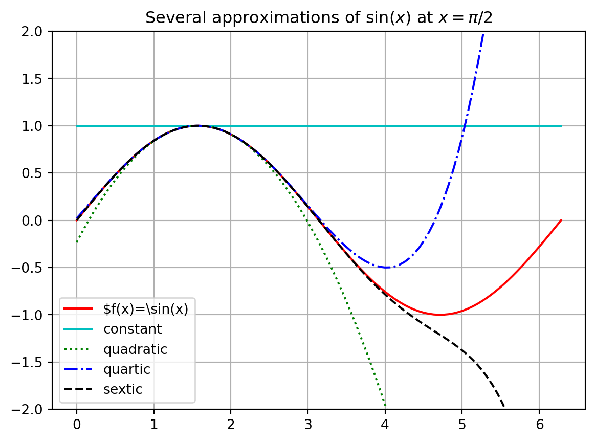
Exercise 2.34 Let us compute a few Taylor Series that are not centred at $x_0 = 0$. For example, let us approximate the function $f(x) = \sin(x)$ near $x_0 = \frac{\pi}{2}$. Near the point $x_0 = \frac{\pi}{2}$, the Taylor Series approximation will take the form \[\begin{equation} f(x) = f\left( \frac{\pi}{2} \right) + f'\left( \frac{\pi}{2} \right)\left( x - \frac{\pi}{2} \right) + \frac{f''\left( \frac{\pi}{2} \right)}{2!}\left( x - \frac{\pi}{2} \right)^2 + \frac{f'''\left( \frac{\pi}{2} \right)}{3!}\left( x - \frac{\pi}{2} \right)^3 + \cdots \end{equation}\]

Write the first several terms of the Taylor Series for $f(x) = \sin(x)$ centred at $x_0 = \frac{\pi}{2}$. Then write Python code to build the plot below showing successive approximations for $f(x) = \sin(x)$ centred at $\pi/2$.

Figure 2.2: Taylor series approximation of the sine function.

Exercise 2.35 Repeat the previous exercise for the function \[ f(x) = \log(x) \text{ centered at } x_0 = 1. \] Use this to give an approximate value for $\log(1.1)$.

Example 2.6 Let us conclude this brief section by examining an interesting example. Consider the function \[\begin{equation} f(x) = \frac{1}{1-x}. \end{equation}\] If we build a Taylor Series centred at $x_0 = 0$ it is not too hard to show that we get \[\begin{equation} f(x) = 1 + x + x^2 + x^3 + x^4 + x^5 + \cdots \end{equation}\] (you should stop now and verify this!). However, if we plot the function $f(x)$ along with several successive approximations for $f(x)$ we find that beyond $x=1$ we do not get the correct behaviour of the function (see Figure 2.3). More specifically, we cannot get the Taylor Series to change behaviour across the vertical asymptote of the function at $x=1$. This example is meant to point out the fact that a Taylor Series will only ever make sense near the point at which you centre the expansion. For the function $f(x) = \frac{1}{1-x}$ centred at $x_0 = 0$ we can only get good approximations within the interval $x \in (-1,1)$ and no further.

Code

import numpy as np
import math as ma
import matplotlib.pyplot as plt

# build the x and y values
x = np.linspace(-1,2,101)
y0 = 1/(1-x)
y1 = 1 + 0*x
y2 = 1 + x
y3 = y2 + x**2
y4 = y3 + x**3 + x**4 + x**5 + x**6 + x**7 + x**8

# plot each of the functions 
plt.plot(x, y0, 'r-', label=r"$f(x)=\sin(x)")
plt.plot(x, y1, 'c-', label=r"constant")
plt.plot(x, y2, 'g:', label=r"linear")
plt.plot(x, y3, 'b-.', label=r"quadratic")
plt.plot(x, y4, 'k--', label=r"8th order")

# set limits on the y axis
plt.ylim(-3,5)

# put in a grid, legend, title, and axis labels
plt.grid()
plt.legend()
plt.title("Taylor approximations of $f(x)=1/(1-x)$ around $x=0$")
plt.show()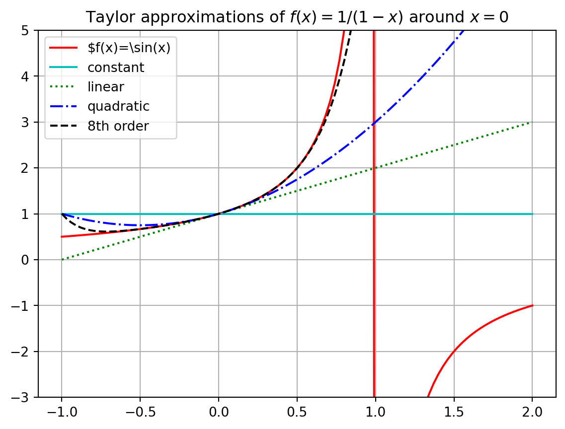

Figure 2.3: Several Taylor Series approximations of the function $f(x) = 1/(1-x)$.

In the previous example we saw that we cannot always get approximations from Taylor Series that are good everywhere. For every Taylor Series there is a domain of convergence where the Taylor Series actually makes sense and gives good approximations. While it is beyond the scope of this section to give all of the details for finding the domain of convergence for a Taylor Series, a good heuristic is to observe that a Taylor Series will only give reasonable approximations of a function from the centre of the series to the nearest asymptote. The domain of convergence is typically symmetric about the centre as well. For example:

If we were to build a Taylor Series approximation for the function $f(x) = \log(x)$ centred at the point $x_0 = 1$ then the domain of convergence should be $x \in (0,2)$ since there is a vertical asymptote for the natural logarithm function at $x=0$.
If we were to build a Taylor Series approximation for the function $f(x) = \frac{5}{2x-3}$ centred at the point $x_0 = 4$ then the domain of convergence should be $x \in (1.5, 6.5)$ since there is a vertical asymptote at $x=1.5$ and the distance from $x_0 = 4$ to $x=1.5$ is 2.5 units.
If we were to build a Taylor Series approximation for the function $f(x) = \frac{1}{1+x^2}$ centred at the point $x_0 = 0$ then the domain of convergence should be $x \in (-1,1)$. This may seem quite odd (and perhaps quite surprising!) but let us think about where the nearest asymptote might be. To find the asymptote we need to solve $1+x^2 = 0$ but this gives us the values $x = \pm i$. In the complex plane, the numbers $i$ and $-i$ are 1 unit away from $x_0 = 0$, so the “asymptote” is not visible in a real-valued plot but it is still only one unit away. Hence the domain of convergence is $x \in (-1,1)$. You may want to pause now and build some plots to show yourself that this indeed appears to be true.

A Taylor Series will give good approximations to the function within the domain of convergence, but will give garbage outside of it. For more details about the domain of convergence of a Taylor Series you can refer to the Taylor Series section of the online Active Calculus Textbook [2].

2.5 Truncation Error

The great thing about Taylor Series is that they allow for the representation of potentially very complicated functions as polynomials – and polynomials are easily dealt with on a computer since they involve only addition, subtraction, multiplication, division, and integer powers. The down side is that the order of the polynomial is infinite. Hence, every time we use a Taylor series on a computer we are actually going to be using is a Truncated Taylor Series where we only take a finite number of terms. The idea here is simple in principle:

If a function $f(x)$ has a Taylor Series representation it can be written as an infinite sum.
Computers cannot do infinite sums.
So stop the sum at some point $n$ and throw away the rest of the infinite sum.
Now $f(x)$ is approximated by some finite sum so long as you stay pretty close to $x = x_0$,
and everything that we just chopped off of the end is called the remainder for the finite sum.

Let us be a bit more concrete about it. The Taylor Series for $f(x) = e^x$ centred at $x_0 = 0$ is \[\begin{equation} e^x = 1 + x + \frac{x^2}{2!} + \frac{x^3}{3!} + \frac{x^4}{4!} + \cdots. \end{equation}\]

$0^{th}$ Order Approximation of $f(x) = e^x$:: If we want to use a zeroth-order (constant) approximation $f_0(x)$ of the function $f(x) = e^x$ then we only take the first term in the Taylor Series and the rest is not used for the approximation \[\begin{equation} e^x = \underbrace{1}_{\text{$0^{th}$ order approximation}} + \underbrace{x + \frac{x^2}{2!} + \frac{x^3}{3!} + \frac{x^4}{4!} + \cdots}_{\text{remainder}}. \end{equation}\] Therefore we would approximate $e^x$ as $e^x \approx 1=f_0(x)$ for values of $x$ that are close to $x_0 = 0$. Furthermore, for small values of $x$ that are close to $x_0 = 0$ the largest term in the remainder is $x$ (since for small values of $x$ like 0.01, $x^2$ will be even smaller, $x^3$ even smaller than that, etc). This means that if we use a $0^{th}$ order approximation for $e^x$ then we expect our error to be about the same size as $x$. It is common to then rewrite the truncated Taylor Series as \[\begin{equation} \text{$0^{th}$ order approximation: } e^x \approx 1 + \mathcal{O}(x) \end{equation}\] where $\mathcal{O}(x)$ (read “Big-O of $x$”) tells us that the expected error for approximations close to $x_0 = 0$ is about the same size as $x$.
$1^{st}$ Order Approximation of $f(x) = e^x$:: If we want to use a first-order (linear) approximation $f_1(x)$ of the function $f(x) = e^x$ then we gather the $0^{th}$ order and $1^{st}$ order terms together as our approximation and the rest is the remainder \[\begin{equation} e^x = \underbrace{1 + x}_{\text{$1^{st}$ order approximation}} + \underbrace{\frac{x^2}{2!} + \frac{x^3}{3!} + \frac{x^4}{4!} + \cdots}_{\text{remainder}}. \end{equation}\] Therefore we would approximate $e^x$ as $e^x \approx 1+x=f_1(x)$ for values of $x$ that are close to $x_0 = 0$. Furthermore, for values of $x$ very close to $x_0 = 0$ the largest term in the remainder is the $x^2$ term. Using Big-O notation we can write the approximation as \[\begin{equation} \text{$1^{st}$ order approximation: } e^x \approx 1 + x + \mathcal{O}(x^2). \end{equation}\] Notice that we do not explicitly say what the coefficient is for the $x^2$ term. Instead we are just saying that using the linear function $y=1+x$ to approximate $e^x$ for values of $x$ near $x_0=0$ will result in errors that are of the order of $x^2$.
$2^{nd}$ Order Approximation of $f(x) = e^x$:: If we want to use a second-order (quadratic) approximation $f_2(x)$ of the function of $f(x) = e^x$ then we gather the $0^{th}$ order, $1^{st}$ order, and $2^{nd}$ order terms together as our approximation and the rest is the remainder \[\begin{equation} e^x = \underbrace{1 + x + \frac{x^2}{2!}}_{\text{$2^{nd}$ order approximation}} + \underbrace{\frac{x^3}{3!} + \frac{x^4}{4!} + \cdots}_{\text{remainder}}. \end{equation}\] Therefore we would approximate $e^x$ as $e^x \approx 1+x+\frac{x^2}{2}=f_2(x)$ for values of $x$ that are close to $x_0 = 0$. Furthermore, for values of $x$ very close to $x_0 = 0$ the largest term in the remainder is the $x^3$ term. Using Big-O notation we can write the approximation as \[\begin{equation} \text{$2^{nd}$ order approximation: } e^x \approx 1 + x + \frac{x^2}{2} + \mathcal{O}(x^3). \end{equation}\] Again notice that we do not explicitly say what the coefficient is for the $x^3$ term. Instead we are just saying that using the quadratic function $y=1+x+\frac{x^2}{2}$ to approximate $e^x$ for values of $x$ near $x_0=0$ will result in errors that are of the order of $x^3$.

Keep in mind that this sort of analysis is only good for values of $x$ that are very close to the centre of the Taylor Series. If you are making approximations that are too far away then all bets are off.

For the function $f(x) = e^x$ the idea of approximating the amount of approximation error by truncating the Taylor Series is relatively straight forward: if we want an $n^{th}$ order polynomial approximation $f_n(x)$ of the function of $f(x)=e^x$ near $x_0 = 0$ then \[\begin{equation} e^x = 1 + x + \frac{x^2}{2!} + \frac{x^3}{3!} + \frac{x^4}{4!} + \cdots + \frac{x^n}{n!} + \mathcal{O}(x^{n+1}), \end{equation}\] meaning that we expect the error to be of the order of $x^{n+1}$.

Exercise 2.36 Now make the previous discussion a bit more concrete. You know the Taylor Series for $f(x) = e^x$ around $x=0$ quite well at this point so use it to approximate the values of $f(0.1) = e^{0.1}$ and $f(0.2)=e^{0.2}$ by truncating the Taylor series at different orders. Because $x=0.1$ and $x=0.2$ are pretty close to the centre of the Taylor Series $x_0 = 0$, this sort of approximation is reasonable.

Then compare your approximate values to Python’s values $f(0.1)=e^{0.1} \approx$ np.exp(0.1) $=1.1051709180756477$ and $f(0.2)=e^{0.2} \approx$ np.exp(0.2) $=1.2214027581601699$ to calculate the truncation errors $\epsilon_n(0.1)=|f(0.1)-f_n(0.1)|$ and $\epsilon_n(0.2)=|f(0.2)-f_n(0.2)|$.

Fill in the blanks in the table. If you want to create the table in your jupyter notebook, you can use Pandas as described in Section 1.7. Alternatively feel free to use a spreadsheet instead of using Python.

Order $n$	$f_n(0.1)$	$\epsilon_n(0.1)=\|f(0.1)-f_n(0.1)\|$	$f_n(0.2)$	$\epsilon_n(0.2)=\|f(0.2)-f_n(0.2)\|$
0	1	1.051709e-01	1	2.214028e-01
1	1.1	5.170918e-03	1.2
2	1.105
3
4
5

You will find that, as expected, the truncation errors $\epsilon_n(x)$ decrease with $n$ but increase with $x$.

Exercise 2.37 To investigate the dependence of the truncation error $\epsilon_n(x)$ on $n$ and $x$ a bit more, add an extra column to the table from the previous exercise with the ratio $\epsilon_n(0.2) / \epsilon_n(0.1)$.

Order $n$	$\epsilon_n(0.1)$	$\epsilon_n(0.2)$	$\epsilon_n(0.2) / \epsilon_n(0.1)$
0	1.051709e-01	2.214028e-01	2.105171
1	5.170918e-03
2
3
4
5

Formulate a conjecture about how $\epsilon_n$ changes as $x$ changes.

Exercise 2.38 To test your conjecture, examine the truncation error for the sine function near $x_0 = 0$. You know that the sine function has the Taylor Series centred at $x_0 = 0$ as \[\begin{equation} f(x) = \sin(x) = x - \frac{x^3}{3!} + \frac{x^5}{5!} - \frac{x^7}{7!} + \cdots. \end{equation}\] So there are only approximations of odd order. Use the truncated Taylor series to approximate $f(0.1)=\sin(0.1)$ and $f(0.2)=\sin(0.2)$ and use Python’s values np.sin(0.1) and np.sin(0.2) to calculate the truncation errors $\epsilon_n(0.1)=|f(0.1)-f_n(0.1)|$ and $\epsilon_n(0.2)=|f(0.2)-f_n(0.2)|$.

Complete the following table:

Order $n$	$\epsilon_n(0.1)$	$\epsilon_n(0.2)$
1	1.665834e-04	1.330669e-03
3	8.331349e-08	2.664128e-06
5	1.983852e-11
7
9

The entry in the last row of the table will almost certainly not agree with your conjecture. That is okay! That discrepancy has a different explanation. Can you figure out what it is? Hint: does np.sin(x) give you the exact value of $\sin(x)$?

Exercise 2.39 Perform another check of your conjecture by approximating $\log(1.02)$ and $\log(1.1)$ from truncations of the Taylor series around $x=1$: \[ \log(1+x) = x - \frac{x^2}{2} + \frac{x^3}{3} - \frac{x^4}{4} + \frac{x^5}{5} - \cdots. \]

Exercise 2.40 Write down your observations about how the truncation error at order $n$ changes as $x$ changes. Explain this in terms of the form of the remainder of the truncated Taylor series.

2.6 Problems

These problem exercises will let you consolidate what you have learned so far and combine it with the coding skills you picked up in Chapter 1.

Exercise 2.41 (This problem is modified from (Greenbaum and Chartier 2012))
Sometimes floating point arithmetic does not work like we would expect (and hope) as compared to by-hand mathematics. In each of the following problems we have a mathematical problem that the computer gets wrong. Explain why the computer is getting these wrong.

Mathematically we know that $\sqrt{5}^2$ should just give us 5 back. In Python type np.sqrt(5)**2 == 5. What do you get and why do you get it?
Mathematically we know that $\left( \frac{1}{49} \right) \cdot 49$ should just be 1. In Python type (1/49)*49 == 1. What do you get and why do you get it?
Mathematically we know that $e^{\log(3)}$ should just give us 3 back. In Python type np.exp(np.log(3)) == 3. What do you get and why do you get it?
Create your own example of where Python gets something incorrect because of floating point arithmetic.

Exercise 2.42 (This problem is modified from (Greenbaum and Chartier 2012))
In the 1999 film Office Space, a character creates a program that takes fractions of cents that are truncated in a bank’s transactions and deposits them to his own account. This idea has been attempted in the past and now banks look for this sort of thing. In this problem you will build a simulation of the program to see how long it takes to become a millionaire.

Assumptions:

Assume that you have access to 50,000 bank accounts.
Assume that the account balances are uniformly distributed between $100 and $100,000.
Assume that the annual interest rate on the accounts is 5% and the interest is compounded daily and added to the accounts, except that fractions of cents are truncated.
Assume that your illegal account initially has a $0 balance.

Your Tasks:

Explain what the code below does.

import numpy as np
accounts = 100 + (100000-100) * np.random.rand(50000,1);
accounts = np.floor(100*accounts)/100;

By hand (no computer) write the mathematical steps necessary to increase the accounts by (5/365)% per day, truncate the accounts to the nearest penny, and add the truncated amount into an account titled “illegal.”
Write code to complete your plan from part (b).
Using a while loop, iterate over your code until the illegal account has accumulated $1,000,000. How long does it take?

Exercise 2.43 (This problem is modified from (Greenbaum and Chartier 2012))
In the 1991 Gulf War, the Patriot missile defence system failed due to roundoff error. The troubles stemmed from a computer that performed the tracking calculations with an internal clock whose integer values in tenths of a second were converted to seconds by multiplying by a 24-bit binary approximation to $\frac{1}{10}$: \[\begin{equation} 0.1_{10} \approx 0.00011001100110011001100_2. \end{equation}\]

Convert the binary number above to a fraction by hand (common denominators would be helpful).
The approximation of $\frac{1}{10}$ given above is clearly not equal to $\frac{1}{10}$. What is the absolute error in this value?
What is the time error, in seconds, after 100 hours of operation?
During the 1991 war, a Scud missile travelled at approximately Mach 5 (3750 mph). Find the distance that the Scud missile would travel during the time error computed in (c).

Exercise 2.44 Find the Taylor Series for $f(x) = \frac{1}{\log(x)}$ centred at the point $x_0 = e$. Then use the Taylor Series to approximate the number $\frac{1}{\log(3)}$ to 4 decimal places.

Exercise 2.45 In this problem we will use Taylor Series to build approximations for the irrational number $\pi$.

Write the Taylor series centred at $x_0=0$ for the function \[\begin{equation} f(x) = \frac{1}{1+x}. \end{equation}\]
Now we want to get the Taylor Series for the function $g(x) = \frac{1}{1+x^2}$. It would be quite time consuming to take all of the necessary derivatives to get this Taylor Series. Instead we will use our answer from part (a) of this problem to shortcut the whole process.
1. Substitute $x^2$ for every $x$ in the Taylor Series for $f(x) = \frac{1}{1+x}$.
2. Make a few plots to verify that we indeed now have a Taylor Series for the function $g(x) = \frac{1}{1+x^2}$.
Recall from Calculus that \[\begin{equation} \int \frac{1}{1+x^2} dx = \arctan(x). \end{equation}\] Hence, if we integrate each term of the Taylor Series that results from part (b) we should have a Taylor Series for $\arctan(x)$.¹
Now recall the following from Calculus:

$\tan(\pi/4) = 1$
so $\arctan(1) = \pi/4$
and therefore $\pi = 4\arctan(1)$.

Let us use these facts along with the Taylor Series for $\arctan(x)$ to approximate $\pi$: we can just plug in $x=1$ to the series, add up a bunch of terms, and then multiply by 4. Write a loop in Python that builds successively better and better approximations of $\pi$. Stop the loop when you have an approximation that is correct to 6 decimal places.

Exercise 2.46 In this problem we will prove the famous (and the author’s favourite) formula \[\begin{equation} e^{i\theta} = \cos(\theta) + i \sin(\theta). \end{equation}\] This is known as Euler’s formula after the famous mathematician Leonard Euler. Show all of your work for the following tasks.

Write the Taylor series for the functions $e^x$, $\sin(x)$, and $\cos(x)$.
Replace $x$ with $i\theta$ in the Taylor expansion of $e^x$. Recall that $i = \sqrt{-1}$ so $i^2 = -1$, $i^3 = -i$, and $i^4 = 1$. Simplify all of the powers of $i\theta$ that arise in the Taylor expansion. I will get you started: \[\begin{equation} \begin{aligned} e^x &= 1 + x + \frac{x^2}{2} + \frac{x^3}{3!} + \frac{x^4}{4!} + \frac{x^5}{5!} + \cdots \\ e^{i\theta} &= 1 + (i\theta) + \frac{(i\theta)^2}{2!} + \frac{(i\theta)^3}{3!} + \frac{(i\theta)^4}{4!} + \frac{(i\theta)^5}{5!} + \cdots \\ &= 1 + i\theta + i^2 \frac{\theta^2}{2!} + i^3 \frac{\theta^3}{3!} + i^4 \frac{\theta^4}{4!} + i^5 \frac{\theta^5}{5!} + \cdots \\ &= \ldots \text{ keep simplifying ... } \ldots \end{aligned} \end{equation}\]
Gather all of the real terms and all of the imaginary terms together. Factor the $i$ out of the imaginary terms. What do you notice?
Use your result from part (c) to prove that $e^{i\pi} + 1 = 0$.

Exercise 2.47 In physics, the relativistic energy of an object is defined as \[\begin{equation} E_{rel} = \gamma mc^2 \end{equation}\] where \[\begin{equation} \gamma = \frac{1}{\sqrt{1 - \frac{v^2}{c^2}}}. \end{equation}\] In these equations, $m$ is the mass of the object, $c$ is the speed of light ($c \approx 3 \times 10^8$m/s), and $v$ is the velocity of the object. For an object of fixed mass (m) we can expand the Taylor Series centred at $v=0$ for $E_{rel}$ to get \[\begin{equation} E_{rel} = mc^2 + \frac{1}{2} mv^2 + \frac{3}{8} \frac{mv^4}{c^2} + \frac{5}{16} \frac{mv^6}{c^4} + \cdots. \end{equation}\]

What do we recover if we consider an object with zero velocity?
Why might it be completely reasonable to only use the quadratic approximation \[\begin{equation} E_{rel} = mc^2 + \frac{1}{2} mv^2 \end{equation}\] for the relativistic energy equation?²
(some physics knowledge required) What do you notice about the second term in the Taylor Series approximation of the relativistic energy function?
Show all of the work to derive the Taylor Series centred at $v = 0$ given above.

Exercise 2.48 (The Python Caret Operator) Now that you’re used to using Python to do some basic computations you are probably comfortable with the fact that the caret, ^, does NOT do exponentiation like it does in many other programming languages. But what does the caret operator do? That’s what we explore here.

Consider the numbers $9$ and $5$. Write these numbers in binary representation. We are going to use four bits to represent each number (it is OK if the first bit happens to be zero). \[\begin{equation} \begin{aligned} 9 &=& \underline{\hspace{0.2in}} \, \underline{\hspace{0.2in}} \, \underline{\hspace{0.2in}} \, \underline{\hspace{0.2in}} \\ 5 &=& \underline{\hspace{0.2in}} \, \underline{\hspace{0.2in}} \, \underline{\hspace{0.2in}} \, \underline{\hspace{0.2in}} \end{aligned} \end{equation}\]
Now go to Python and evaluate the expression 9^5. Convert Python’s answer to a binary representation (again using four bits).
Make a conjecture: How do we go from the binary representations of $a$ and $b$ to the binary representation for Python’s a^b for numbers $a$ and $b$? Test and verify your conjecture on several different examples and then write a few sentences explaining what the caret operator does in Python.

There are many reasons why integrating an infinite series term by term should give you a moment of pause. For the sake of this problem we are doing this operation a little blindly, but in reality we should have verified that the infinite series actually converges uniformly.↩︎
This is something that people in physics and engineering do all the time – there is some complicated nonlinear relationship that they wish to use, but the first few terms of the Taylor Series captures almost all of the behaviour since the higher-order terms are very very small.↩︎

Order \(n\)	\(\epsilon_n(0.1)\)	\(\epsilon_n(0.2)\)	\(\epsilon_n(0.2) / \epsilon_n(0.1)\)
0	1.051709e-01	2.214028e-01	2.105171
1	5.170918e-03
2
3
4
5