Appendix A — Solutions
This appendix holds the solutions to selected exercises in the book. Please look at these solutions only after having made a serious attempt at solving the exercises and knowing exactly where you got stuck.
A.1 Continuous-time population models
Von Bertalanffy growth
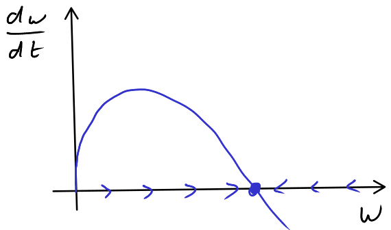
- Seeking a steady state we find \(\alpha w^{2/3}-\beta w = 0\) \(\implies\) \(w^{2/3}(\alpha-\beta w^{1/3})=0\) \(\implies\) \(w=0\) or \(w^{1/3} = \alpha/\beta\). With the graphical approach in Figure A.1 we see that the non-zero steady state is stable. Hence, \[ \lim_{t \rightarrow \infty} w(t) = \left( \frac{\alpha}{\beta} \right)^{3}. \tag{A.1}\]
For the time derivative of \(u=w^{1/3}\) we find by the chain rule that \[ \frac{du}{dt} = \frac13 w^{-2/3} \frac{dw}{dt} = \frac{1}{3u^2}\left( \alpha w^{2/3}-\beta w \right). \tag{A.2}\] Hence \[ 3\frac{du}{dt} = \frac{1}{u^2}\left( \alpha u^2-\beta u^3 \right) = \alpha-\beta u. \tag{A.3}\] So this change of variables has yielded a linear first-order ODE with constant coefficients, which is easy for us to solve: \[ u(t) = \frac{1}{\beta} \left( \alpha - Ae^{-\beta t/3}\right) \tag{A.4}\] for some integration constant \(A\). If \(u(0)=u_0\) then \(A=\alpha -\beta u_0\).
Translating back to \(w\) with \(w_0=u_0^3\) we finally have \[ w(t) = u(t)^3 = \frac{1}{\beta^3}\left( \alpha - \left( \alpha - \beta w_0^{1/3} \right) e^{-\beta t/3} \right)^3. \tag{A.5}\]
Solving logistic equation
Exercise 1.3: We separate the variables by dividing both sides of the ODE by \(N(1-N/K)\) and multiplying by \(dt\), and then integrate to get \[ \int_{N_0}^{N(t)}\frac{dN}{N\left(1-\frac{N}{K}\right)}=\int_0^t r\,dt. \tag{A.6}\] The right hand side is trivial to integrate, but for the integral on the left-hand side we need to employ the method of partial fractions, using that \[ \frac{dN}{N\left(1-\frac{N}{K}\right)}=\frac{1}{N}+\frac{1}{K-N}. \tag{A.7}\] The left-hand side then gives \[ \begin{split} \int_{N_0}^{N(t)}&\left(\frac{1}{N}+\frac{1}{K-N(t)}\right)dN\\ &=\log N(t)-\log N_0-\log(K-N(t))+\log(K-N_0). \end{split} \tag{A.8}\] We exponentiate both sides to get \[ \frac{N(t)}{N_0}\frac{K-N_0}{K-N(t)}=e^{rt}. \tag{A.9}\] Now we just need to solve for \(N(t)\): \[ N(t)=\frac{N_0Ke^{rt}}{K+N_0(e^{rt}-1)}. \tag{A.10}\]
Harvesting with fixed quota
**Exercise 1.5: If we harvest with a fixed quota \(Q\), the population is described by the equation \[ \frac{dN}{dt} = \alpha N \log\frac{K}{N} - Q. \tag{A.11}\] The subtraction of \(Q\) shifts the graph of the right-hand side down by a distance \(Q\). This brings the non-zero fixed points closer together until \(Q\) is equal to the maximum of the growth rate of the unfished population. If \(Q\) is increased beyond this value the non-zero fixed points disappear and the population will go extinct. is because we are removing \(Q\) individuals from the population at a constant rate. Thus the maximum sustainable yield occurs when \(Q\) equals the maximum replenishment rate of the unfished population. To find that maximum we first solve \[ 0=\frac{d}{dN}\left(\alpha N \log\frac{K}{N}\right)=\alpha\left(\log\frac{K}{N}-1\right). \tag{A.12}\] This tells us that the maximum is at \[ N_{max} = K\,e^{-1}. \tag{A.13}\] Hence the value at the maximum is \[ MSY=Q_{max}=\alpha N_{max} \log\frac{K}{N_{max}}=\alpha\,K\,e^{-1}. \tag{A.14}\] Fishing at this quota is not wise, as this reduces the population to the threshold level below which the population will go extinct.
Wasp model
Exercise 1.6: For \(0\leq t\leq t_c\) the number of workers satisfies \[ \frac{dn}{dt}=r\,n. \tag{A.15}\] Therefore \[ n(t)=n_0e^{r\,t}. \tag{A.16}\]
For \(t_c\leq t\leq T\) the number of reproducers satisfies \[ \frac{dN}{dt}=Rn(t_c)=R\,n_0\,e^{r\,t_c}, \tag{A.17}\] so that \[ N(T)=(T-t_c)R\,e^{r\,t_c}. \tag{A.18}\]
To find the value of \(t_c\) that maximises \(N(T)\) we set the derivative of \(N(T)\) with respect to \(t_c\) to zero: \[ \begin{split} 0&=\frac{d}{dt_c}N(T)=\frac{d}{dt_c}(T-t_c)R\,e^{r\,t_c}\\ &=-R\,e^{r\,t_c}+(T-t_c)R\,r\,e^{r\,t_c}\\ &=R\,e^{r\,t_c}(r\,T-r\,t_c-1). \end{split} \tag{A.19}\] This implies that \[ t_c=T-\frac{1}{r}. \tag{A.20}\]
Wasp model with death
Exercise 1.7: For \(0\leq t\leq t_c\) the number of workers satisfies \[ \frac{dn}{dt}=(r-d)n. \tag{A.21}\] Therefore \[ n(t)=e^{(r-d)t}. \tag{A.22}\] For \(t_c\leq t\leq T\) we have \[ \frac{dn}{dt}=-dn \tag{A.23}\] so that \[ n(t)=n(t_c)e^{-d(t-t_c)}=e^{(r-d)t}e^{-d(t-t_c)}=e^{r\,t_c}e^{-d\,t}. \tag{A.24}\] Also for \(t_c\leq t\leq T\) the number of reproducers satisfies \[ \frac{dN}{dt}=Rn(t)=Re^{r\,t_c}e^{-d\,t}, \tag{A.25}\] so that \[ N(T)=\int_{t_c}^TRe^{r\,t_c}e^{-d\,t}dt = \frac{R}{d}e^{r\,t_c}\left(e^{-d\,t_c}-e^{-d\,T}\right). \tag{A.26}\] To find the value of \(t_c\) that maximises \(N(T)\) we set the derivative of \(N(T)\) with respect to \(t_c\) to zero: \[ \begin{split} 0&=\frac{d}{dt_c}N(T)=\frac{d}{dt_c}\left( \frac{R}{d}e^{r\,t_c}\left(e^{-d\,t_c}-e^{-d\,T}\right)\right)\\ &=Re^{r\,t_c}\left(\left(\frac{r}{d}-1\right)e^{-d\,t_c}-\frac{r}{d}e^{-d\,T}\right). \end{split} \tag{A.27}\] This is equivalent to \[ e^{-d\,t_c}=\frac{1}{1-d/r}e^{-d\,T} \tag{A.28}\] and thus \[ t_c=T+\frac{1}{d}\ln\left(1-\frac{d}{r}\right). \tag{A.29}\]
A.2 Discrete-time population models
Verhulst model
Exercise 2.1: Let’s write the equation as \(N_{t+1}=f(N_t)\) with \[ f(N)=rN\left(1-\frac{N}{K}\right). \tag{A.30}\]
Because \(f(N)\) is positive for all \(N<K\), the only way for \(N_{t+1}\) to be negative is for \(N_t\) to be greater than \(K\). This in turn is only possible if \(f(N_{t-1})>K\). So the function \(f\) at its maximum needs to be larger than \(K\). Because the function describes an upside-down parabola with zeros at \(0\) and \(K\), its maximum is in the middle at \(N=K/2\), where \(f(K/2)=rK/4\). Thus the population can get negative iff \(rK/4>K\), which is equivalent to \(r>4\).
A.3 Sex-structured population models
Dominance structure
- The ratio \(F/Q\) in the negative term in the equation for the alpha females represents the fact that if the ratio between the subordinate individuals who gather the food and the alpha females who rely on that food is too small, then the alpha females don’t get enough food and hence are less fit, leading to either a decreased birth rate or an increased mortality rate.
We derive the ODE: \[\begin{split} \frac{d}{dt}\frac{F}{Q }&=\frac{F'Q -FQ'}{Q ^2}\\ &= \frac{(b_F-\mu_F F/Q )F Q-F(b_Q F-\mu_Q Q )}{Q ^2}\\ &=(b_F+\mu_Q )\frac{F}{Q }\left(1-\frac{b_Q +\mu_F}{b_F+\mu_Q }\frac{F}{Q }\right). \end{split} \tag{A.31}\] Ideally you identify this as the logistic equation with initial growth rate \(r\) and carrying capacity \(K\) given by \[ r=b_F+\mu_Q ,~~~K=\frac{b_F+\mu_Q }{b_Q +\mu_F}. \tag{A.32}\] You can then look up the solution in the lecture notes: \[ \frac{F}{Q }(t)=\frac{\frac{F_0}{Q_0}Ke^{rt}}{K+\frac{F_0}{Q_0}\left(e^{rt}-1\right)}. \tag{A.33}\] Otherwise you have to work a bit harder.
Because we have identified \(F/Q (t)\) as the solution of a logistic equation it is easy to see that as \(t\to\infty\), \(F/Q \to K\) with \(K\) as in Eq. A.32.
We derive the ODE: \[\begin{split} \frac{d}{dt}\frac{F}{M}&=\frac{F'M-FM'}{M^2}\\ &= \frac{(b_F-\mu_F F/Q )FM-F(b_MF-\mu_M M)}{M^2}\\ &=\frac{F}{M}\left(b_F+\mu_M-\mu_F\frac{F}{Q }-b_M\frac{F}{M}\right). \end{split} \tag{A.34}\] We are only interested in the limit of \(F/M\) as \(t\to\infty\). Let us denote this limit by \(R\). We already know that the limit of \(F/Q\) as \(t\to\infty\) is \(K\). The limit of the previous equation gives \[ 0=\frac{d}{dt}R=R\left(b_F+\mu_M-\mu_FK-b_MR\right) \tag{A.35}\] and hence \[ R=\frac{b_F+\mu_M-\mu_FK}{b_M}. \tag{A.36}\] Substituting the expression for \(K\) and bringing everything on a common denominator gives \[ R=\frac{(b_F+\mu_M)(b_Q +\mu_F)-\mu_F(b_F+\mu_Q )}{b_M(b_Q +\mu_F)} \tag{A.37}\] To see that this is always positive we multiply out the numerator: \[ R=\frac{b_Fb_Q +\mu_Mb_Q +\mu_M\mu_F-\mu_F\mu_Q }{b_M(b_Q +\mu_F)} \tag{A.38}\] This is positive because \(b_Fb_Q >\mu_F\mu_Q\)
The birth rates are linear in the number of alpha females and independent of \(M\) and \(Q\). Independence of \(M\) is realistic only if \(M\) is large. Using a weighted mean might be better, i.e., birth rates given by \(b_i FM/(F/n+M)\), where \(n\) is the number of females a male can mate with per mating season. Or we could take into account that the alpha females will reproduce less if there are fewer subordinate individuals gathering food for them, for example by choosing birth rates to be given by \(b_i F Q/(F/n+Q )\), where \(n\) is the number of pregnant females that a subordinate monkey can keep well fed. There are many other possible improvements.
A.4 Age-structured population models
Harvestings an age-structured population
Exercise 4.2: We can start from Eq. 4.14 that gives the expected number of offspring produced by an individual within their lifetime: \[ \phi(0) = \int_0^\infty b(a) \exp\left(-\int_0^a \mu(a') \, da'\right)\, da. \tag{A.39}\] This will now simplify when we use the given expressions Eq. 4.46 and Eq. 4.47 for the rates. Because \(b(a)\) is non-zero only for \(a>a_m\), the outer integral only has to run from \(a_m\) to \(\infty\). The inner integral from \(0\) to \(a\) we need to split into two integrals because of the piece-wise nature of \(\mu(a)\). Hence \[ \phi(0) = \int_{a_m}^\infty b(a) \exp\left(-\int_0^{a_m} \mu(a') \, da' -\int_{a_m}^a \mu(a') \, da'\right)\, da. \tag{A.40}\] We can now substitute the appropriate constants for the rates: \[ \begin{split} \phi(0) &= \int_{a_m}^\infty b\, \exp\left(-\int_0^{a_m} \mu_0 \, da' -\int_{a_m}^a (\mu_0+\mu_F) \, da'\right)\, da\\ &= \int_{a_m}^\infty b\, \exp\left(-\mu_0 a_m - (\mu_0+\mu_F)(a-a_m)\right)\, da\\ &= b\,\exp(-\mu_F a_m) \int_{a_m}^\infty \, \exp\left(- (\mu_0+\mu_F)a\right)\, da\\ &= b\,\exp(-\mu_F a_m) \left[-\frac{1}{\mu_0+\mu_F}\exp\left(- (\mu_0+\mu_F)a\right)\right]_{a_m}^\infty\\ &= b\,\exp(-\mu_F a_m) \frac{1}{\mu_0+\mu_F}\exp\left(- (\mu_0+\mu_F)a_m\right)\\ &= \frac{b}{\mu_0+\mu_F}\exp\left(-\mu_0a_m\right). \end{split} \tag{A.41}\] This expected number of offspring produced by an individual within their lifetime must be greater or equal to \(1\) for the population to sustain itself. Hence the upper limit on the harvesting rate \(\mu_F\) is given by \[ \mu_F \leq b\exp\left(-\mu_0a_m\right) - \mu_0. \tag{A.42}\]
Seasonal mortality
Substituting \(n(t,a)=p(t)r(a)\) into Eq. 4.3 and dividing by \(n(t,a)\) gives \[ \frac{p'(t)}{p(t)}+\frac{r'(a)}{r(a)}=-\mu(a)-f(t). \tag{A.43}\] Separating variables gives \[ \frac{p'(t)}{p(t)}+f(t)=-\frac{r'(a)}{r(a)}-\mu(a). \tag{A.44}\] As the left-hand side is independent of \(a\) and the right-hand side is independent of \(t\), both sides must be equal to some constant \(\gamma\). This gives us the two ODEs \[ \frac{d}{dt}\log(p(t))=\gamma-f(t),~~~\frac{d}{da}\log(r(a))=-\gamma-\mu(t). \tag{A.45}\] These have the solutions \[ \begin{split} p(t)&=p(0)\exp\left(\int_0^t\gamma-f(s)\,ds\right),\\ r(a)&=r(0)\exp\left(-\int_0^a\gamma+\mu(s)\,ds\right) \end{split} \tag{A.46}\] Thus the solution for \(n\) is \[ n(t,a)=n(0,0)\exp\left(\int_0^t\gamma-f(s)\,ds\right) \exp\left(-\int_0^a\gamma+\mu(s)\,ds\right). \tag{A.47}\]
Substituting the solution into Eq. 4.4 gives \[ p(t)r(0)=\int_0^\infty b(a)p(t)r(a)\,da. \tag{A.48}\] After dividing by \(p(t)r(0)\) and using our expression for \(r(a)\) from the previous part, \[ 1=\int_0^\infty b(a) \exp\left(-\int_0^a\gamma+\mu(s)ds\right)da =\phi(\gamma). \tag{A.49}\] The factor \(\exp(-\gamma a)\) in the integrand decreases monotonically with increasing \(\gamma\) and therefore so does the integral. Hence the function \(\phi(\gamma)\) is a monotonically decreasing function.
The end of a season occurs at any \(t\in\mathbb{Z}\). At those integer times we can write the integral in the expression for \(p(t)\) as \[ \begin{split} \int_0^t\gamma-f(s)\,ds&=\sum_{i=1}^t\int_{i-1}^{i}\gamma-f(s)\,ds\\ &=\sum_{i=1}^t(\gamma - F)=t(\gamma - F). \end{split} \tag{A.50}\] Hence for the population at the end of the season \(t\) we have \[ n(t,a)=n(0,0)\exp(t(\gamma - F))r(a). \tag{A.51}\] This will go to zero in the limit \(t\to\infty\) if \(\gamma - F<0\). Thus the criterion for extinction is \(\gamma < F\).
Because \(\phi(\gamma)\) decreases with \(\gamma\), \[ \gamma < F \Leftrightarrow \phi(\gamma) > \phi(F). \tag{A.52}\] Because \(\phi(\gamma)=1\), this is equivalent to the condition \(1>\phi(F)\). Thus the condition for extinction is \[ \int_0^\infty b(a) \exp\left(-\int_0^a F+\mu(s)\,ds\right)da <1. \tag{A.53}\]
A.5 Interacting populations
A.6 Epidemics
SIR with recrudescence
Exercise 6.2: The modified equations are \[ \begin{split} \frac{dS}{dt} &= -\beta S I/N,\\ \frac{dI}{dt} &= \beta S I/N - \gamma I + \delta R,\\ \frac{dR}{dt} &= \gamma I - \delta R. \end{split} \tag{A.54}\]
At the steady state all these derivatives have to vanish. From the first equation we find \(S^*=0\) or \(I^*=0\). We are not interested in \(I^*=0\) because we are interested in the endemic state which by definition has \(I^*>0\), so we have \(S^*=0\). The third equation gives \(R^*=\gamma/\delta I^*\). Then \(I^*\) is found from the fact that \(N=S^*+I^*+R^*\) which gives \(I^*=N-\gamma/\delta I^*\). Soving for \(I^*\) gives \[ I^*=\frac{N\delta}{\delta+\gamma}. \tag{A.55}\]
For the stability analysis we reduce the problem to a two-dimensional system by eliminating \(S\) from the last two equations. This gives \[ \begin{split} \frac{dI}{dt} &= \frac{\beta I}{N} \left(N-I-R\right) - \gamma I + \delta R,\\ \frac{dR}{dt} &= \gamma I - \delta R. \end{split} \tag{A.56}\] The Jacobian matrix is \[ A = \begin{pmatrix} \frac{\beta}{N} \left(N-2I-R\right) -\gamma & \delta-\frac{\beta I}{N}\\ \gamma & -\delta \end{pmatrix}. \tag{A.57}\] Evaluated at the endemic state this gives \[ A = \begin{pmatrix} -\frac{\beta}{N}I^* -\gamma & \delta-\frac{\beta}{N}I^*\\ \gamma & -\delta \end{pmatrix}. \tag{A.58}\] This has determinant and trace given by \[ \begin{split} \det(A) &= (\delta+\gamma)\frac{\beta}{N}I^*>0,\\ \text{tr}(A) &= -\frac{\beta}{N}I^* -\gamma -\delta <0. \end{split} \tag{A.59}\] so the endemic state is stable for all positive values of the parameters.
SIR model with reinfections
Exercise 6.3: The modified equations are \[ \begin{split} \frac{dS}{dt} &= -\beta S I/N,\\ \frac{dI}{dt} &= \beta S I/N - \gamma I +\beta\mu R I/N,\\ \frac{dR}{dt} &= \gamma I-\beta\mu R I/N. \end{split} \tag{A.60}\] At the steady state all these derivatives have to vanish. From the first equation we find \(S^*=0\) or \(I^*=0\). We are not interested in \(I^*=0\) because we are interested in the endemic state which by definition has \(I^*>0\), so we have \(S^*=0\). The third equation gives \(R^*=\gamma N/(\beta\mu)\). Then \(I^*\) is found from the fact that \(N=S^*+I^*+R^*\) which gives \[ I^*=N-R^*=N\left(1-\frac{\gamma}{\beta\mu}\right). \tag{A.61}\] This is not the same as the number of infecteds in the endemic state of the model with loss of immunity given in Eq. 6.33.
Sex-structured SIR model
As \(N=S+I+R\) we have \[ \frac{dN}{dt} = \frac{dS}{dt}+\frac{dI}{dt}+\frac{dR}{dt} = -rSI'+rSI'-aI+aI=0. \tag{A.62}\] Hence, \(N\) is a constant. Similarly, \(N'\) is a constant.
We start by deriving an ODE for \(S\) as a function of \(R'\): \[ \frac{dS}{dR'}=\frac{dS}{dt}/ \frac{dR'}{dt} = \frac{-rSI'}{a'I'}=-\frac{r}{a'}S. \tag{A.63}\] This is easy to solve: \[ S(t)=S_0e^{-\frac{r}{a'}R'(t)}. \tag{A.64}\] Similarly, \[ S'(t)=S'_0e^{-\frac{r'}{a}R(t)}. \tag{A.65}\]
At \(t=\infty\) we have \[ S(\infty)=S_0 e^{-\frac{r}{a'}R'(\infty)}. \tag{A.66}\] But at \(t=\infty\), \(I'=0\) and \(N'=S'+I'+R'\) and so \[ S(\infty)=S_0 e^{-\frac{r}{a'}(N'-S'(\infty))}. \tag{A.67}\] Similarly, \[ S'(\infty)=S'_0 e^{-\frac{r'}{a}(N-S(\infty))}. \tag{A.68}\]
A.7 Spatially-structured population models
Fishing model with diffusion
The spatially uniform steady states are \(F^*=0\) and \(K\). Stability can be determined graphically or from the gradient at the steady state, with the result that \(F^*=0\) is unstable and \(F^*=K\) is stable.
If \(F\) is small then \(\frac{\partial F}{\partial t} \approx rF + D\frac{\partial^2 F}{\partial x^2}\).
Try \(F(x,t) = e^{\lambda t}\left( A \cos k x + B\sin k x \right)\) such that \[ \frac{\partial F}{\partial x} = k e^{\lambda t}\left( -A \sin k x + B\cos k x \right). \tag{A.69}\] The boundary conditions are \(F(0,t) = 0 = \frac{\partial F}{\partial x}(L,t)\). The boundary condition at \(x=0\) implies that \(A=0\). The second implies that \[ \cos kL = 0\implies k = \frac{(2n+1)\pi }{2L} =: k_n, ~~~ n = 0,~1,~2,.... \tag{A.70}\] Substituting this solution into the PDE gives \[ \lambda = \lambda_n =: r-k_n^2D. \tag{A.71}\]
A full solution is a superposition of the above solutions. For the fish population not to collapse we need at least one \(\lambda_n>0\) for some \(n\). The largest \(\lambda_n\) is for the smallest \(k_n\), which occurs when \(n=0\), giving the requirement that \(\lambda_0 = r-D\left( \frac{\pi}{2L}\right)^2>0\). Hence, we need \[ L^2>\frac{D\pi^2}{4r}. \tag{A.72}\]
Travelling wave in 1-species reaction-diffusion model
With \(z=x-ct\) we have \[ \frac{\partial }{\partial t}= \frac{\partial z}{\partial t}\frac{\partial }{\partial z} = -c \frac{\partial }{\partial z} \text{ and } \frac{\partial }{\partial x}= \frac{\partial z}{\partial x}\frac{\partial }{\partial z} = \frac{\partial }{\partial z}. \tag{A.73}\] Substituting this into the PDE gives the ODE \[ -cU' = f(U) + DU''. \tag{A.74}\]
For a travelling wave from left to right (\(c>0\)) we expect solution at \(\pm \infty\) to be at steady state: \(U(-\infty) = 1\) and \(U(\infty)=0\), with \(U'(\pm \infty)=0\).
We will now use a slightly different way to approach the linearisation around the leading edge of the travelling wave than the one we used in the lecture. The methods are equivalent, and it is always instructional to look at different ways of doing the same thing.
At the leading edge of the wave we have that \(U\) is very small, so we can Taylor-expand \(f(U)=f(0)+Uf'(0)+\dots\). We keep only the first two terms and also use that \(f(0)=0\) to get the linear ODE \[ -cU' = Uf'(0)+DU''. \tag{A.75}\] Rather than making an Ansatz for \(U\) as in the lecture, we convert this second order ODE into a set of first-order ODEs by introducing a second variable \(V\) so that \(U'=V\) and \(V' = -\frac{U}{D}f'(0) - \frac{c}{D}V\). In vector notation this reads \[ \begin{pmatrix} U'\\ V' \end{pmatrix} = \begin{pmatrix} 0 & 1\\ -\frac{f'(0)}{D}U & -\frac{c}{D} \end{pmatrix} \begin{pmatrix} U\\ V \end{pmatrix}. \tag{A.76}\] The eigenvalues \(\lambda\) of this linear matrix ODE are solutions of \[ \det \begin{pmatrix} -\lambda & 1 \\ -\frac{f'(0)}{D} & -\lambda -\frac{c}{D} \end{pmatrix} = 0 ~~~~\implies ~~~~\lambda^2 + \frac{c}{D} \lambda + \frac{f'(0)}{D}=0. \tag{A.77}\] Real eigenvalues and thus realistic biological solutions exist iff \[ \frac{c^2}{D^2}-4\frac{f'(0)}{D}\geq 0, ~~~~\implies ~~~~ c\geq 2\sqrt{Df'(0)}. \tag{A.78}\]
If \(f(u)= 0\) for all \(u\) we get \(DU''+cU'=0\). Setting \(U(z)=e^{\mu z}\) \(\implies\) \(D\mu^2+c\mu\) \(\implies\) \(\mu = 0\) or \(-c/D\). The general solution is \(U=Ae^{-\frac{c}{D} z}+B\). Clearly \(|U|\rightarrow \infty\) as \(z \rightarrow -\infty\). This is not a biologically realistic solution.
SIR model with logistic growth
One can either approach this systematically or one can just try to guess the necessary change of variables. We will use a blended approach: we guess the expressions for \(u\) and \(v\) by inspecting the equations, and we make a general Ansatz for \(\tilde{t}\).
By comparing the \((1-S/K)\) factor in the equation for \(S\) to the factor \((1-u)\) in the equation for \(u\) we see that \(u=S/K\). It is natural to also choose \(v=I/K\). We write \(\tilde{t}=t/\tau\), where \(\tau\) is still to be determined. With these we have \[\begin{split} \partial_{\tilde{t}}u&=\tau/K\partial_tS= \tau/K\left(rKu(1-u)-\beta K^2uv\right)\\ &= \tau r u(1-u)-\tau \beta K uv \end{split} \tag{A.79}\] By comparing this with equation for \(u\) in the problem statement, we can read off that \[ \tau = \frac{1}{\beta K}, ~~~b=\frac{r}{\beta K}. \tag{A.80}\] Then \[\begin{split} \partial_{\tilde{t}}v&=\tau/K\partial_tI= \tau/K\left(\beta K^2uv-\gamma Kv\right)\\ &=uv-\frac{\gamma}{\beta K}v. \end{split} \tag{A.81}\] By comparing this with the equation for \(v\) in the problem statement we read off that \[ m=\frac{\gamma}{\beta K}. \tag{A.82}\]
By inspection we see that one steady state is \((u(x,t),v(x,t))=(0,0)\) and that another is \[ (u(x,t),v(x,t))=(1,0). \tag{A.83}\] The first describes a situation where the foxes are extinct, the second the situation where in the absence of the disease the fox population sits at its carrying capacity. We look for another steady state \((u(x,t),v(x,t))=(u^*,v^*)\) with \(v^*\neq 0\). From the equation for \(v\) we read off that \(u^*=m\) and then from the equation for \(u\) we get \(v^*=b(1-m)\). This is the endemic state because the number of infecteds is nonzero. It exists as long as \(m<1\). This tells us that the existence of the endemic state is independent of the intrinsic growth rate \(r\) of the fox population but does depend on its carrying capacity.
We know from part a. that \(\partial_{\tilde t}u=\partial_t I/(\beta K^2)\). Thus we now want \(D_1\partial_x^2 S/(\beta K^2)=\partial_{\tilde{x}}^2 u\), where \(u=S/K\). Hence \[ \tilde{x}=\sqrt{\frac{K\beta}{D_1}}x. \tag{A.84}\] Then \(d\,\partial_{\tilde{x}}^2v =d\,D_1\partial_x^2I\) but we want \(D_2\partial_x^2I\) so we need \[ d=\frac{D_2}{D_1}. \tag{A.85}\]
Substituting the wave Ansatz into the PDEs for \(u\) and \(v\) gives \[\begin{split} -cA'&=bA(1-A)-AB+A''\\ -cB'&=AB-mB+dB''. \end{split} \tag{A.86}\]
If \(A(\infty)=1\) (which corresponds to \(S=K\)) then that means that at \(x=\infty\) the system is in the disease-free state and thus \(B(\infty)=0\). At \(x=-\infty\) the system must thus be in the endemic state, so \(A(-\infty)=u^*=m\) and \(B(-\infty)=v^*=b(1-m)\). So the key to this question was the observation that the travelling wave will always have to interpolate between two steady states.
At the leading edge where \(B\) is very small, \(A\) is very close to \(1\), so \(A=1-\epsilon\) for a small \(\epsilon>0\). The equations Eq. A.86 can thus be approximated by the linear equations \[ c\epsilon'=b\epsilon-B-\epsilon'',~~~-cB'=B-mB+dB''. \tag{A.87}\] We obtained this by dropping all terms involving \(\epsilon^2\) or \(\epsilon B\) because they are negligible when \(\epsilon\) and \(B\) are both small.
We concentrate on the second equation, which we solve with the Ansatz \(B(x)=\exp(\lambda x)\). Substituting this Ansatz into the equation gives the characteristic equation for \(\lambda\): \[ d\lambda^2+c\lambda+1-m=0, \tag{A.88}\] and thus \[ \lambda=\frac{-c\pm\sqrt{c^2-4d(1-m)}}{2d}. \tag{A.89}\] We do not want the solution to oscillate, so we want \(\lambda\) to be real, hence \[ c\geq 2\sqrt{d(1-m)}. \tag{A.90}\]
Derive Turing instability
Here, \[ f(u,v)=a-u + u^2v, ~~~~ g(u,v)=b-u^2v. \tag{A.91}\]
Step 1. Uniform steady state
\[ a-u^* + {u^*}^2 v^*=0~\text{ and }~b-{u^*}^2 v^*=0 \tag{A.92}\] implies \[ (u^*,~v^*)=(a+b,~b/(a+b)^2). \tag{A.93}\]
Step 2. Linearize
Set \(u=u^*+\xi\) and \(v=v^*+\eta\) with \(\xi\) and \(\eta\) small. Substitute and Taylor expand to get \[ \begin{pmatrix} \frac{\partial \xi}{\partial t} \\ \frac{\partial \eta}{\partial t} \end{pmatrix} = \begin{pmatrix} a_{11} & a_{12} \\a_{21} & a_{22} \end{pmatrix} \begin{pmatrix} \xi \\ \eta \end{pmatrix} + \begin{pmatrix} D_1 \frac{\partial^2 \xi}{\partial x^2} \\ D_2\frac{\partial^2 \eta}{\partial x^2} \end{pmatrix}, \tag{A.94}\] where \[ \begin{split} a_{11} = \frac{\partial f}{\partial u}(u^*,v^*) &= -1+2u^*v^* \\ &= -1+2(a+b)b/(a+b)^2 \\ &=(b-a)/(a+b)\\ a_{12} = \frac{\partial f}{\partial v}(u^*,v^*) &= {u^*}^2 =(a+b)^2\\ a_{21} = \frac{\partial g}{\partial u}(u^*,v^*) &= -2 u^* v^* =-2b/(a+b)\\ a_{22} = \frac{\partial g}{\partial v}(u^*,v^*) &= -{u^*}^2 =-(a+b)^2 \end{split} \tag{A.95}\]
Step 3. Solutions
Make the Ansatz \(\xi = A_1 e^{\sigma t} \sin( kx+\alpha)\) and \(\eta = A_2 e^{\sigma t} \sin( kx+\alpha)\). Substitute to get \[ \begin{pmatrix} \sigma - \frac{b-a}{a+b} +D_1k^2 & -(a+b)^2 \\ \frac{2b}{a+b} & \sigma + (a+b)^2 +D_2k^2 \end{pmatrix} \begin{pmatrix} A_1 \\ A_2 \end{pmatrix}= {\mathbf 0} \tag{A.96}\] For a non-trivial solution we require the determinant of this matrix to be zero (otherwise we would be able to find an inverse, etc.). Hence, \[ \sigma^2 + \left[ (a+b)^2 - \frac{b-a}{a+b} + (D_1+D_2)k^2 \right] \sigma + h(k^2) = 0, \tag{A.97}\] where \[ h(k^2)= D_1D_2k^4 - \left[ D_2\frac{b-a}{a+b} - D_1(a+b)^2 \right] k^2 +(a+b)^2. \tag{A.98}\]
Step 4. In the absence of diffusion (Put \(D_1=0=D_2\).) \[ \sigma^2 + \left[ (a+b)^2 - \frac{b-a}{a+b} \right] \sigma + (a+b)^2 = 0. \tag{A.99}\] For \(\sigma\) to have roots in the left half of the complex plane (giving us a stable steady state) we need \((a+b)^2-\frac{b-a}{a+b}>0 ~\implies ~ b-a<(a+b)^3\) and \((a+b)^2>0\) (which it is).
Step 5. With diffusion (\(D_1\neq 0\neq D_2\).)
We want steady state to be unstable in this case. The coefficient of \(\sigma\) is \[ (a+b)^2 - \frac{b-a}{a+b} + (D_1+D_2)k^2 > (D_1+D_2)k^2>0 ~~~~\mbox{from Step 4} \tag{A.100}\] Therefore, we require \(h(k^2)<0\) for some \(k^2\) for there to be an instability.
As \(h(0)>0\) we must have two positive real roots of \(h(k^2)=0\) for there to be an instability.
Real distinct roots (\(\implies ~~B^2-4AC>0\)) \[ \implies \left[ D_2\frac{b-a}{a+b} - D_1(a+b)^2 \right]^2> 4D_1D_2 (a+b)^2. \tag{A.101}\] Both positive (\(\implies B<0\)) \[ \implies D_2\frac{b-a}{a+b} - D_1(a+b)^2 > 0. \tag{A.102}\]
Slime mould with boundary
Exercise 7.7 \[ \frac{\partial a}{\partial t} = \frac{\partial}{\partial x} \left( \mu \frac{\partial a}{\partial x} - \chi a \frac{\partial \rho}{\partial x} \right), ~~~\mbox{and} ~~~ \frac{\partial \rho}{\partial t} = fa -k\rho + D\frac{\partial^2 \rho}{\partial x^2}. \tag{A.103}\] Steady states are \(fa^*=k\rho^*\).
Consider a perturbation \(a=a^*+\xi\) and \(\rho = \rho^* +\eta\), where \(\xi\) and \(\eta\) are small. Substitute and linearize to give \[ \frac{\partial \xi}{\partial t} = \mu \frac{\partial^2 \xi}{\partial x^2} - \chi a^* \frac{\partial^2 \eta}{\partial x^2}, ~~~\mbox{and} ~~~ \frac{\partial \eta}{\partial t} = f\xi -k\eta + D\frac{\partial^2 \eta}{\partial x^2}. \tag{A.104}\] Put \(\xi = A_1 e^{\sigma t + iqx}\) and \(\eta = A_2 e^{\sigma t + iqx}\). Hence, \[ \begin{pmatrix} \sigma +\mu q^2 & -\chi a^*q^2 \\ -f & \sigma + k+Dq^2 \end{pmatrix} \begin{pmatrix} A_1 \\ A_2 \end{pmatrix}= {\mathbf 0} \tag{A.105}\]
A non-trivial solution requires the determinant of the matrix to be zero \[ \implies ~\sigma^2 +g(q^2)\sigma + h(q^2) = 0, \tag{A.106}\] where \(g(q^2) = k+(D+\mu)q^2>0\) and \(h(q^2) = \mu Dq^4+(k\mu -\chi a^*f)q^2>0\).
We need \((k\mu -\chi a^*f)<0\) for there to be a positive root of \(h(q^2)=0\) and so instability.
If \(0\leq x \leq L\) we need boundary conditions. Assume no flux at \(x=0,~L\): \(\frac{\partial a}{\partial x}=0=\frac{\partial \rho}{\partial x}\) at \(x=0,~L\).
Try \(\xi = A_1 e^{\sigma t}\cos qx\) and \(\eta = A_2 e^{\sigma t}\cos qx\) to satisfy BCs at \(x=0\).
At \(x=L\) we have \(\sin qL = 0\) for a non-trivial solution \(~\implies q=q_n:= n\pi/L\), \(n=0,1,2,...\)
Aggregation will not occur if \(h(q_1^2)>0\), which implies \[ L<\pi\sqrt{\frac{D\mu}{\chi a^*f-k\mu}}. \tag{A.107}\]
Aggregation will occur if \[ k\mu<\chi a^*f ~~~\mbox{and}~~~ L>\pi\sqrt{\frac{D\mu}{\chi a^*f-k\mu}}. \tag{A.108}\]