2 Discrete-time population models

So far we have assumed that the rate of change of the population number has no explicit time dependence. However births and also deaths often happen on an annual cycle. Many fish have their spawning season in the spring, and many birds breed in the summer and annual plants produce their seed and then die in winter. In this case, the rate of change of the population number is not constant, but depends on the time of the year. We can model this by introducing a time dependence in the birth and death rates. However this will lead to equations that will be difficult to analyse. Instead we can give up on the idea of modelling the population numbers continuously through time and instead only follow how the population changes from year to year.

So we will use models of the form \[ N_{t+1} = f(N_t) \tag{2.1}\] where $N_t$ is the population number at time $t$ and $f$ is some function. Time $t$ now takes on only integer values, and the population number is only defined at these times. This is called a discrete-time model. Given the initial population number $N_0$, we can calculate the population number at any future time $t$ by iterating the function $f$: $N_1 = f(N_0)$, $N_2 = f(N_1)=f(f(N_0)),\ldots N_t = f(f(\ldots f(N_0)\ldots))$.

2.1 Exponential model

The simplest discrete-time model is the exponential model \[ N_{t+1} = R N_t \tag{2.2}\] where $R>0$ is the growth factor. This is the discrete-time version of the continuous-time exponential model. The solution to this equation is \[ N_t = N_0 R^t. \tag{2.3}\] It is important to stress that $R$ is not a growth rate but a dimensionless growth factor. Comparing the discrete-time solution to the continuous-time solution $N(t)=N_0\exp(rt)$ we see that they agree at integer times $t$ if we measure time in years and set \[ R=\exp(r \cdot 1\text{ year}). \tag{2.4}\] If you are confused by the units, remember that the exponential function is dimensionless, so the argument of the exponential function must be dimensionless. We need the extra factor of 1 year because $r$ is a rate and has dimension 1/time.

The population number grows exponentially with time if $R>1$ and declines exponentially if $R<1$. To get more realistic models we again need to introduce a limited carrying capacity.

2.2 Models with limited carrying capacity

Recall how we introduced the logistic model by assuming that the per-capita birth rate declines linearly with the population number and vanishes when the population reaches its carrying capacity. This gave us the equation \[ \frac{dN}{dt} = rN\left(1 - \frac{N}{K}\right) \tag{2.5}\] where $r$ is the per-capita growth rate and $K$ is the carrying capacity.

It turns out that there are several models which all deserve to be called the discrete-time logistic model.

2.2.1 Verhulst model

The most famous discrete-time logistic model is the Verhulst model.

\[ \begin{split} N_{t+1} &= (R_0+1)N_t\left(1 - \frac{N_t}{K(R_0+1)/R_0}\right)\\ &=N_t + R_0 N_t\left(1 - \frac{N_t}{K}\right)=f(N_t). \end{split} \tag{2.6}\] Again it is important to stress that $R_0$ is not a growth rate but a dimensionless growth factor.

We have written the model in two alternative forms because the first form makes the analogy with the continuous-time logistic model more obvious, while the second form makes it easier to read off the fixed point.

The fixed point is a value for which $N_{t+1}=N_t$, i.e. a value of $N$ for which the population number does not change from year to year. Thus it is a value $N^*$ for which $f(N^*)=N^*$. Using the second form of the model, we can see easily that the fixed points are $N^*=0$ and $N^*=K$, so $K$ is the carrying capacity.

A problem with the Verhulst model is that it can give rise to negative population numbers. This is not realistic, so we are motivated to modify the model to prevent this.

2.2.2 Ricker model

The Ricker model is a modification of the Verhulst model that prevents negative population numbers. It is given by \[ N_{t+1} = N_t\, e^{R_0\left(1 - \frac{N_t}{K}\right)}. \tag{2.7}\] By moving the logistic factor inside the exponential, the Ricker model prevents negative population numbers. The fixed points are still $N^*=0$ and $N^*=K$. Ricker introduced this model to describe salmon populations.

2.2.3 Beverton-Holt model

The Beverton-Holt model is another modification of the Verhulst model which prevents negative population numbers. It is given by \[ N_{t+1} = \frac{R N_t}{1 + \frac{R-1}{K}N_t}. \tag{2.8}\] This has been a very influential model in fisheries science. On the face of it the model does not look very similar to the logistic model, but we will see the relationship when we solve the model. The Beverton-Holt model is one of the rare cases where a non-linear model can be solved exactly. The trick is to make a change of variables from $N_t$ to $u_t = 1/N_t$. Then we have \[ u_{t+1} = \frac{1}{N_{t+1}} = \frac{1 + \frac{R-1}{K}N_t}{R N_t} = \frac{u_t}{R} + \frac{R-1}{R K}. \tag{2.9}\] This is a linear equation for $u_t$, and linear equations are easy to solve. The easiest way to proceed is to look at the first few terms of the sequence $u_t$ and guess the general form of the solution. We find \[\begin{split} u_1 &= \frac{u_0}{R} + \frac{R-1}{R K},\\ u_2 &= \frac{u_0}{R^2} + \frac{R-1}{R K}\left(1 + \frac{1}{R}\right),\\ u_3 &= \frac{u_0}{R^3} + \frac{R-1}{R K}\left(1 + \frac{1}{R} + \frac{1}{R^2}\right),\\ &\vdots\\ u_t &= \frac{u_0}{R^t} + \frac{R-1}{R K}\left(1 + \frac{1}{R} + \frac{1}{R^2} + \ldots + \frac{1}{R^{t-1}}\right). \end{split} \tag{2.10}\] The sum in the second term is a geometric series. We know the general formula for a geometric series: \[ 1 + x + x^2 + \ldots + x^{t-1} = \frac{1 - x^t}{1 - x}. \tag{2.11}\]

We can use this with $x=1/R$ to sum terms in the second term. We find \[ u_t = \frac{u_0}{R^t} + \frac{R-1}{R K}\frac{1 - (1/R)^t}{1 - 1/R}. \] We simplify this a bit and bring everything on the same denominator. \[ u_t = \frac{u_0}{R^t} - \frac{(1/R)^t-1}{K} =\frac{Ku_0-1+R^t}{KR^t}. \tag{2.12}\]

We can now change back to $N_t=1/u_t$ to find the solution to the Beverton-Holt model. We find \[\begin{split} N_t &= \frac{1}{u_t}=\frac{K R^t}{Ku_0-1+R^t}\\ &=\frac{K/u_0}{KR^{-t}-R^{-t}/u_0+1/u_0}\\ &=\frac{KN_0}{N_0+(K-N_0)R^{-t}}. \end{split} \tag{2.13}\]

This is the solution to the Beverton-Holt model. Comparing this to the solution of the continuous-time logistic model \[ N(t) = \frac{KN_0}{N_0+(K-N_0)\exp(-rt)} \tag{2.14}\] we see that they agree at integer times $t$ if we measure time in years and set $R=\exp(r \cdot 1\text{ year}).$

2.3 Stability and Cobwebs

We now want to study the stability of the fixed points in discrete-time models. As discussed, fixed points $N^*$ satisfy the equation $N^*=f(N^*)$. We study the stability of the fixed points by looking at the sequence $N_t$ for $t$ close to the fixed point. That means we write $N(t)=N^*+n_t$ for $n_t<<1$. We then have \[ \begin{split} N_{t+1} = N^*+n_{t+1}=f(N_t) = f(N^*+n_t) = f(N^*) + f'(N^*)n_t + \ldots \end{split} \tag{2.15}\] where we have used the Taylor expansion of $f$ around $N^*$. Because $N^*$ is a fixed point, we have $f(N^*)=N^*$. Thus we find that \[ n_{t+1} \approx f'(N^*)n_t \tag{2.16}\] where we neglected the higher order terms in the Taylor expansion. This is a linear equation for $n_t$ that we know how to solve: \[ n_t = n_0 (f'(N^*))^t. \tag{2.17}\] So we have found that:

If $|f'(N^*)|<1$, then $n_t$ will decrease with time and the fixed point is stable.
If $|f'(N^*)|>1$, then $n_t$ will increase with time and the fixed point is unstable.

If $|f'(N^*)|=1$, then we cannot say anything about the stability of the fixed point from this analysis.

In the continuous-time case we also had a graphical way to see the stability of fixed points. We will now introduce a graphical method for studying the stability of fixed points in discrete-time models, called the cobweb method.

We plot the function $f(N_t)$ and the line $N_{t+1}=N_t$. The fixed points are the intersection points of the function and the line. We then draw the graph of the sequence $N_t$ by starting at the initial population number $N_0$ and iterating the function $f(N_t)$ to find $N_1$, then iterating the function again to find $N_2$, and so on. The graph of the sequence $N_t$ is called the cobweb. The stability of the fixed points can be read off from the cobweb. If the cobweb spirals into the fixed point, as shown in Figure 2.1, then the fixed point is stable. If the cobweb spirals out of the fixed point, as shown in Figure 2.2, then the fixed point is unstable. You have to press the play button below the figures to see the cobweb diagrams in action.

Figure 2.1: Cobweb diagram for a stable fixed point.

Figure 2.2: Cobweb diagram for an unstable fixed point.

The oscillatory nature of the sequence $N_t$, hopping from one side of the fixed point to the other, that creates the cobweb pattern is due to the fact that the slope of $f$ is negative at the fixed point. The graphical method for visualising the iterations will work also when the slope is positive at the fixed point, but it will not look like a cobweb. Figure 2.3 shows the cobweb for a stable fixed point with positive slope.

Figure 2.3: Cobweb diagram for a fixed point with positive slope.

2.4 Discrete-time harvesting model

We will now look at an example of a discrete-time model with harvesting and apply the techniques we have learned. The model has the standard discrete-time model form $N_{t+1}=f(N_t)$, where $f$ in our example is \[ f(N) = \frac{b N^2}{1+N^2}-EN. \] The constant $b>2$ determines the growth rate of the population and the harvesting rate is determined by the harvesting effort $E$.

We start by studying the model without harvesting, so we set $E=0$ for now. As usual, we start by looking at the steady states of the model. The fixed points are the solutions to the equation \[ N^* = \frac{b\,{N^*}^2}{1+{N^*}^2}. \] There is the obvious solution $N^*=0$. We can then find the non-zero solutions by dividing both sides by $N^*$ and multiply them by $1+{N^*}^2$ to get the equation \[ 1+{N^*}^2 = bN^*. \] This is a quadratic equation for $N^*$, which we could rewrite in the more convential form \[ {N^*}^2 - bN^* + 1 = 0. \] The solutions to this equation are \[ N^*_\pm = \frac{b\pm\sqrt{b^2-4}}{2}. \] The solutions are real if $b^2-4\geq 0$, i.e. if $b\geq 2$, which we have stipulated earlier. Both solutions are positive.

We now have enough information to draw a good sketch to understand the dynamics of the model. We can draw the function $f(N)$ and the line $N_{t+1}=N_t$. It may not be immediately obvious what the sketch of $f(N)=bN^2/(1+N^2)$ looks like. We’ll reason ourselves through this in steps:

First let us consider what happens near $N=0$. There the function is approximately $f(N)\approx bN^2$. This is a parabola that opens upwards. The function is zero at $N=0$ and increases quadratically with $N$.
Next we consider what happens as $N$ becomes large. There the function is approximately $f(N)\approx b$. So the graph has a horizontal asymptote at $y=b$.
We know that in between there are two fixed points. That means the graph needs to cross the diagonal line $y=N$ twice.
Finally we observe that the function is monotonically increasing.

If we now draw something that has all these features, we will have a sufficiently good sketch of the function for our purpose of understanding the dynamics of the model. We will necessarily end up with something that qualitatively looks like the graph in Figure 2.4.

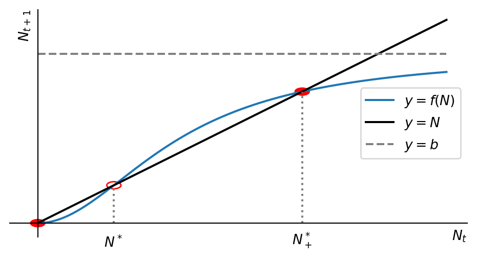
Figure 2.4: Graph of the function $f(N)=\frac{bN^2}{1+N^2}$.

Using our cobweb technique, or simply looking at the slope of $f$ at the fixed points, we can easily convince ourselves that the extinction fixed point is stable, the smaller non-zero fixed point $N^*_-$ is unstable and the larger fixed point $N^*_+$ is stable. in Figure 2.4 we have indicated the stable fixed points by solid circles and the unstable fixed points by open circles. So when the population number is larger than $N^*_-$ it will grow towards $N^*_+$, and when it is smaller than $N^*_-$ it will go extinct. So this model exhibits a strong Allee effect with critical depensation. $N^*_-$ is the smallest viable population size.

We can now add harvesting to the model. The extra term in the function $f(N)$ is $-EN$. This lowers the graph of $f(N)$ by an amount that grows linearly with $N$. This is illustrated in Figure 2.5.

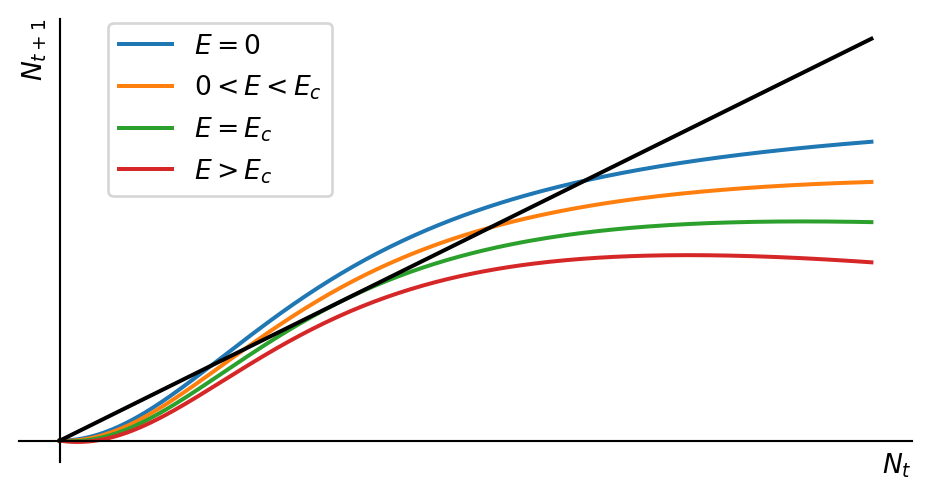
Figure 2.5: Graph of the function $f(N)=\frac{bN^2}{1+N^2}-EN$.

We see that as the harvesting effort $E$ increases, the two fixed points move closer together. At a critical value $E_c$ the two fixed points merge and disappear. The population number will then go extinct for all initial population numbers.

Let us find the critical value $E_c$. For that we first determine the location of the fixed points in the presence of harvesting. So we solve the equation \[ N^* = \frac{b\,{N^*}^2}{1+{N^*}^2}-EN^*. \] Again this has a solution $N^*=0$. We can then find the non-zero solutions by dividing both sides by $N^*$ and multiply them by $1+{N^*}^2$ to get the equation \[ (1+E){N^*}^2-bN^*+1+E = 0. \] This is solved by \[ N^*_\pm = \frac{\frac{b}{1+E}\pm\sqrt{\left(\frac{b}{1+E}\right)^2-4}}{2}. \] We see that these solutions are real only if $\left(\frac{b}{1+E}\right)^2-4\geq 0$, i.e., if $E< \frac{b-2}{2}$. Thus the critical effort is $E_c=\frac{b-2}{2}$. Fishing above this level will lead to extinction of the population. But even fishing just near this level is risky because the population number will be very close to the minimum viable population and a small disturbance could lead to extinction.

2.5 Bifurcations

A bifurcation is a change in the existence and/or stability of the fixed points as the parameters of the model are varied.

You have met bifurcations in continuous-time models already in your Dynamical Systems module. You have seen there that in one-dimensional systems described by a single ODE there are three different types of bifurcation: saddle-node, pitchfork, transcritical. The same types of bifurcations can occur in discrete-time models but there is also one more type: the period-doubling bifurcation.

We have already seen a bifurcation in the discrete-time harvesting model. The bifurcation was a saddle-node bifurcation, where two fixed points merge and disappear. This is also sometimes referred to as a tangent bifurcation, because at the critical value of the parameter the curve $y=f(N)$ is tangent to the line $y=N$ at the fixed point.

In the period-doubling bifurcation the stability of the fixed point changes as the parameter is varied. The fixed point changes from stable to unstable, and at the same time a stable period-2 orbit appears, where the population number oscillates between two values. The period-2 orbit is stable in the sense that if the population number is close to the orbit it will converge to the orbit. This kind of bifurcation can obviously not arise in one-dimensional continuous-time models because a continuous orbit can not move from one side of a fixed point to the other.

In the lectures we drew diagrams illustrating three of the four types of bifurcations. For a discussion of all four types in a similar fashion, you can view the following video.

2.6 Exercises

Exercises marked with a * are essential and are to be handed in. Exercises marked with a + are important and you are urged to complete them. Other exercises are optional but recommended. The exercise marked with an o will be worked through in the problems class.

+ Verhulst model

Exercise 2.1 For some choices of the parameters, the Verhulst model \[N_{t+1}=rN_t\left(1-\frac{N_t}{K}\right) \tag{2.18}\] can lead to negative population numbers even when initially starting with a positive population below its carrying capacity. Derive the condition on the parameters for this to happen. One good way to approach this is to think about what the cobweb diagram would have to look like for such a scenario.

* Ricker model

Exercise 2.2 Find the fixed points in the Ricker model \[ N_{t+1} = N_t\, e^{R_0\left(1 - \frac{N_t}{K}\right)}. \tag{2.19}\] and investigate their stability. Do this both analytically and by drawing cobweb diagrams.

Beverton-Holt model

Exercise 2.3 Find the fixed points in the Beverton-Holt model \[ N_{t+1} = \frac{R N_t}{1 + \frac{R-1}{K}N_t}. \tag{2.20}\] and investigate their stability. Do this both analytically and by drawing cobweb diagrams.

o House finches

Exercise 2.4 [Note: in this problem we combine a continuous time model for the dynamics within a single year with a discrete model for the dynamics from one year to the next. The subscript $t \in \mathbb{Z}$ refers to the discrete year whereas $\tau\in\mathbb{R}$ will indicate the continuous time within a single year.]

A population of house finches resides in an isolated region in North America. In this problem you want to find out about the long-term prospects for the population.

Each year the males and females begin their search for mates at the beginning of winter with a combined population number $N_t$ in year $t$, and form $P_t$ breeding pairs by the end of this search period, the start of the breeding season.

The mate search period lasts from within-year time $\tau = 0$ to the end of the search period at within-year time $\tau = T$. Assume that there is a 1:1 sex ratio and that males $M(\tau)$ and females $F(\tau)$ locate one another randomly to make a pair at rate $\sigma$, such that the number $M(\tau)$ of males that are not in a pair at time $\tau$ satisfies \[\frac{dM}{d\tau}=-\sigma \,M\,F \] and similarly the number $F$ of females that are not in a pair at time $\tau$ satisfies \[\frac{dF}{d\tau}=-\sigma \,M\,F. \]

You are given that the number of breeding pairs that establish a nest and breed successfully is $G(P_t)P_t$, where the fraction $G(P_t)$ takes the particular form \[G(P_t) = \frac{1}{1+P_t/\delta},\] where $\delta$ represents the density of available nesting sites. Each pair that reproduces successfully has a mean number $c$ of offspring.

The probability that a bird will survive from one year to the next is $s$.

Show that the number $n(\tau)=M(\tau)+F(\tau)$ of birds not in a pair is governed by \[\frac{dn}{d\tau}=-\frac{\sigma}{2}n^2, ~~~n(0)=N_t.\]
Using the above, show that the number $n(T)$ of birds that have not found a mate at the start of the breeding season in year $t$ is \[n(T)=\frac{r\,N_t}{r+2N_t}\] where $N_t$ is the number of birds at the start of the season in that particular year and where $r=4/(\sigma T)$.
Explain why the number of pairs $P(\tau)$ is governed by \[\frac{dP}{d\tau}=-\frac12\frac{dn}{d\tau},~~~P(0)=0.\]
Use the above to show that the number of breeding pairs at the start of the breeding season in year $t$ is \[P_t:=P(T)=\frac{N_t^2}{r+2N_t}.\]
Show that the population $N_{t+1}$ at the beginning of winter in year $t+1$ is given by \[ N_{t+1}=s\,N_t+\frac{c\,N_t^2}{r+2N_t+N_t^2/\delta}. \tag{2.21}\]
Find the realistic steady states of the model in Eq. 2.21 for the case that \[\frac{c}{1-s}-2\geq \sqrt{\frac{4r}{\delta}}.\]
Draw a cobweb diagram to illustrate the stability of the steady states in the case that there are two positive steady states. Label key features of the curves.
What type of bifurcation occurs when there is equality in the condition in part f)?

Another model

Exercise 2.5 Consider the discrete time model \[ N_{t+1}=\frac{rN_t}{1+(N_t/K)^b} \tag{2.22}\] where $r$, $b$ and $K$ are positive parameters with $b>1$. Show that the model has two steady states. Investigate the stability of the extinction steady state. Show that the non-trivial (non-zero) steady state can lose stability through a period doubling bifurcation at $b=2r/(r-1)$, or a tangent bifurcation at $r=1$.