mizerSeasonal

After you have installed the mizerSeasonal package with

remotes::install_github("gustavdelius/mizerSeasonal")

you can load it with

library(mizerSeasonal)
#> Loading required package: mizer

We demonstrate the use of the package by introducing seasonal reproduction into the North Sea model that comes with mizer. So we load the model, match its growth rates to observations and run it to steady state:

p <- NS_params |> matchGrowth() |> steady(preserve = "erepro")
#> Convergence was achieved in 13.5 years.
plotlySpectra(p, power = 2)

This is not a particularly good model of the North Sea, but it will suffice for demonstration purposes.

In standard mizer the way to find a good steady state for a model is to first keep the reproduction independent of the rate of investment into reproduction and run the dynamics until it settles down. Then one adapts the reproduction parameters in the model so that the steady-state investment into reproduction leads to the desired steady state reproduction (this is what the steady() function did above). We will follow the same method for the model with seasonal reproduction.

Following the paper by Datta, S. & Blanchard, J. L. “The effects of seasonal processes on size spectrum dynamics”. Canadian Journal of Fisheries and Aquatic Sciences (2016). https://cdnsciencepub.com/doi/full/10.1139/cjfas-2015-0468, we describe the seasonal reproduction rate by the von Mises distribution \[ R_{dd}(t) = r_0 \frac{\exp(\kappa \cos(2\pi(t - \mu)))}{2\pi I_0(\kappa)}, \] which looks like a Gaussian near \(t = \mu\) but is periodic in \(t\) with a period of one year. The spawning season is centred at \(\mu\) with a length proportional to \(1/\sqrt{\kappa}\) and a magnitude determined by \(r_0\). The denominator involving the Bessel function \(I_0\) is just a normalisation factor that makes sure that the integral over \(R_{dd}(t)\) is equal to \(r_0\).

We need to specify the new species parameters \(r_0, \kappa\) and \(\mu\) (which are denoted by rdd_vonMises_r0, rdd_vonMises_kappa and rdd_vonMises_mu respectively). We choose \(r_0\) to be equal to the reproduction rate \(R_{dd}\) of the non-seasonal model and we take \(\mu\) and \(\kappa\) from the paper by Datta et.al.

species_params(p)$rdd_vonMises_r0 <- getRDD(p)
species_params(p)$rdd_vonMises_kappa <- 
    c(3.6047, 2.9994, 1.944, 0.40493, 1.141, 1.4257,
      4.973, 0.795, 4.0495, 3.6567, 5.4732, 1.951)
species_params(p)$rdd_vonMises_mu <- 
    c(0.5477, 0.0643, 0.3574, 0.8576, 0.3825, 0.3716,
      0.4856, 0.5021,0.2245, 0.4181, 0.3123, 0.3333)

We also need to set the mass-specific gonad release rate \(r(t)\) so that mizer can calculate the gonadic mass. Unfortunately we do not know which release rate \(r(t)\) produces the steady-state reproduction rate that we have chosen above. We will try a vonMises distribution with the same \(\kappa\) and \(\mu\) parameters as above and with \(r_0\) chosen large enough so that most of the gonadic mass is released every year. We will then later set the parameters of the Beverton-Holt function to produce the desired reproduction rate.

species_params(p)$vonMises_r0 <- 100
species_params(p)$vonMises_kappa <- species_params(p)$rdd_vonMises_kappa
species_params(p)$vonMises_mu <- species_params(p)$rdd_vonMises_mu

Seasonal reproduction is then turned on with

p <- setSeasonalReproduction(p, release_func = "seasonalVonMisesRelease",
                             RDD = "seasonalVonMisesRDD")

The resulting MizerParams object can be projected into the future as usual with project() to produce a MizerSim object.

sim <- project(p, t_max = 50, dt = 0.01)
plotlyBiomass(sim)

We see that the system has settled down to a steady state quite quickly.

To see the variation within the year we project for a further year but with higher time resolution

ps <- setInitialValues(p, sim)
sim1 <- project(ps, t_max = 1, dt = 0.01, t_save = 0.01)
plotlyBiomass(sim1)

Let us look at an animation of the size spectrum for one year. We first re-run the simulation while storing fewer intermediate times to make the animation render more quickly.

sim1l <- project(ps, t_max = 1, dt = 0.01, t_save = 0.1)
animateSpectra(sim1l, power = 2)

Hit the “Play” button to see the size spectra evolve over the course of a year. Because we are in the steady state, the next year will again look the same, so you can simply play the above simulation repeatedly.

We notice that, while the seasonal reproduction has a big effect on the seasonal variation of the abundance of larvae, the abundance of mature fish remains unaffected. The cohort peaks are damped while they move up the size spectrum and disappear almost completely by the time they reach the maturity size.

As a result, when we animate the gonadic spectrum, i.e., the size distribution of the total gonadic mass of each species, the shape of the distribution does not change much but simply moves up and down during the year due to the seasonal release rate and the constant creation of gonadic mass.

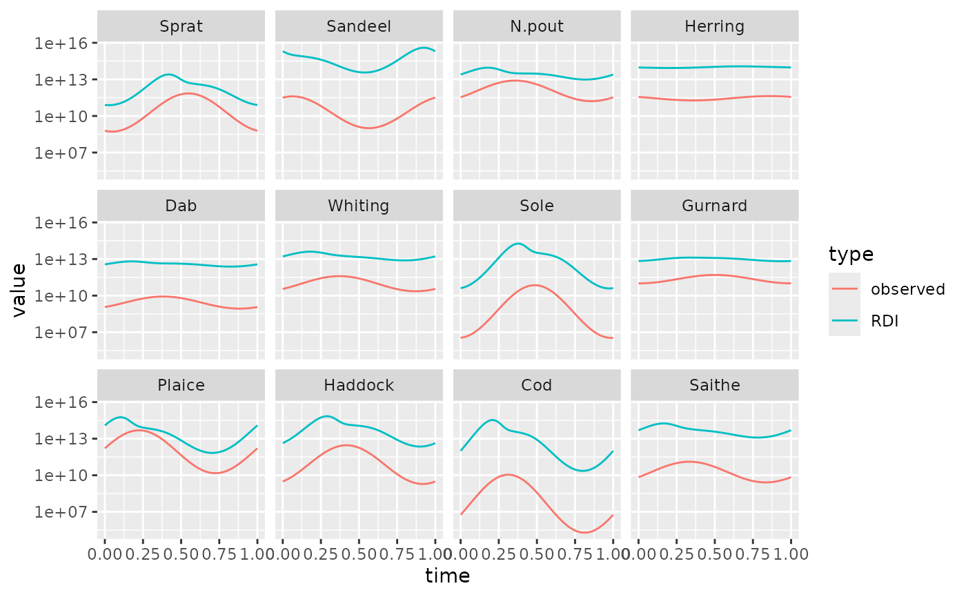
animateGonadSpectra(sim1l)

We can take a look at the rate \(R_{di}\) of reproduction before density dependence and the desired rate \(R_{dd}\) that should remain after imposing an \(R_{max}\). Both vary throughout the year:

rdi <- getTimeseries(sim1, func = getRDI)
rdd <- getTimeseries(sim1, func = getRDD)
# build data frame for ggplot
rdi_df <- melt(rdi)
rdi_df$type <- "RDI"
rdd_df <- melt(rdd)
rdd_df$type <- "observed"
df <- rbind(rdi_df, rdd_df)
# Make plot with one panel per species
library(ggplot2)
ggplot(df) + 
    geom_line(aes(x = time, y = value, colour = type)) +
    facet_wrap(vars(sp)) +
    scale_y_log10()

We now set the maximum reproduction rate \(R_{max}(t)\) so that the density-dependent reproduction \(R_{dd}\) produced by the Beverton Holt function \[ R_{dd} = R_{di}\frac{R_{max}}{R_{di}+R_{max}} \] agrees with the observed reproduction rate.

other_params(ps)$r_max <- rdi * rdd / (rdi - rdd)
ps <- setRateFunction(ps, "RDD", "seasonalBevertonHoltRDD")