Stochastic Gradient Descent Distribution versus Posterior

When we train a statistical model by performing stochastic gradient descent (SGD) on the negative log-likelihood, the stochastic nature of the process means the parameters do not settle at a fixed point. Instead, they keep wandering through parameter space. This document explores the remarkable connection between this wandering and the Bayesian posterior distribution.

We use the same two models introduced in Regular and Singular Models: a regular normal model and a singular Gaussian mixture model.

The SGD Update Rule and Its Noise

Given \(n\) data points \(X = \{x_1, \dots, x_n\}\), the full-batch negative log-likelihood is \[ L_n(w) = -\frac{1}{n} \sum_{i=1}^n \log p(x_i \mid w). \] Full gradient descent updates the parameters deterministically: \[ w_{t+1} = w_t - \eta \, \nabla L_n(w_t). \]

In stochastic gradient descent, we instead pick a random mini-batch \(\mathcal{B}_t \subset \{1, \dots, n\}\) of size \(B\) and use the noisy estimate: \[ \nabla \tilde{L}(w_t) = -\frac{1}{B} \sum_{i \in \mathcal{B}_t} \nabla \log p(x_i \mid w_t). \]

We can decompose this into the true gradient plus noise: \[ \nabla \tilde{L}(w_t) = \nabla L_n(w_t) + \xi_t, \] where \(\xi_t\) is a zero-mean noise term with covariance \[ \text{Cov}(\xi_t) = \frac{C(w_t)}{B}, \quad C(w) = \frac{1}{n} \sum_{i=1}^n \nabla \log p(x_i \mid w) \, \nabla \log p(x_i \mid w)^\top - \nabla L_n(w) \, \nabla L_n(w)^\top. \]

With constant learning rate \(\eta\), SGD does not converge. The noise \(\xi_t\) continuously pushes the parameters away from the minimum. The trajectory forms a random cloud—a stationary distribution in parameter space. What is this distribution?

Continuous-Time SDE Approximation

For small \(\eta\), the discrete SGD update can be approximated by a continuous-time stochastic differential equation (SDE). Near a minimum \(w^*\) of \(L_n\), we linearize the gradient using the Hessian \(H = \nabla^2 L_n(w^*)\): \[ \nabla L_n(w) \approx H (w - w^*). \]

The SGD dynamics then become an Ornstein–Uhlenbeck (OU) process: \[ dw = -\eta \, H (w - w^*) \, dt + \sqrt{\frac{\eta}{B}} \, C^{1/2}(w^*) \, dW_t, \] where \(W_t\) is standard Brownian motion.

The stationary distribution of this OU process is Gaussian: \[ w_\infty \sim \mathcal{N}\!\left(w^*,\; \Sigma\right), \] where the covariance \(\Sigma\) satisfies the continuous Lyapunov equation \[ H \Sigma + \Sigma H = \frac{C(w^*)}{B}. \] If \(H\) and \(C\) are simultaneously diagonalizable (or if we work in the eigenbasis of \(H\)), then \[ \Sigma = \frac{1}{2B} H^{-1} C(w^*). \]

Connection to the Posterior Distribution

Now comes the key insight. In a well-specified model (the true distribution \(q\) lies in the model family), the gradient noise covariance \(C(w^*)\) at the MLE is closely related to the Fisher information matrix, which in turn equals the Hessian \(H\): \[ C(w^*) \approx H. \]

Substituting this into the stationary covariance: \[ \Sigma \approx \frac{1}{2B} H^{-1} H = \frac{1}{2B} I. \]

More precisely, the stationary distribution takes the form \[ \pi_{\text{SGD}}(w) \propto \exp\!\left(-\frac{1}{2} (w - w^*)^\top \Sigma^{-1} (w - w^*)\right) \approx \exp\!\left(-\frac{L_n(w)}{T}\right), \] where the effective temperature is \[ \boxed{T = \frac{\eta}{2B}.} \]

Compare this to the Bayesian posterior with a flat prior: \[ \pi_{\text{post}}(w) \propto \exp\!\left(-n \, L_n(w)\right) = \exp\!\left(-\frac{L_n(w)}{1/n}\right). \]

The posterior corresponds to temperature \(T_{\text{post}} = 1/n\). Therefore, SGD samples from the posterior when \[ \frac{\eta}{2B} = \frac{1}{n}, \quad \text{i.e.,} \quad \eta = \frac{2B}{n}. \]

This is the central result of Mandt, Hoffman & Blei (2017): constant-learning-rate SGD is an approximate Bayesian sampler with temperature controlled by the learning rate and batch size.

NoteStochastic Gradient Langevin Dynamics (SGLD)

Welling & Teh (2011) proposed adding explicit Gaussian noise to SGD to make it a proper MCMC sampler. In SGLD the update is \[ w_{t+1} = w_t - \eta \, \nabla \tilde{L}(w_t) + \sqrt{2\eta / n} \; \epsilon_t, \quad \epsilon_t \sim \mathcal{N}(0, I). \] With a decaying learning rate \(\eta_t \to 0\), the injected noise dominates the mini-batch noise, and the iterates converge to exact posterior samples. At constant \(\eta\), SGLD produces approximate samples just like vanilla SGD, but the injected noise gives more direct control over the temperature.

Model 1: A Regular Statistical Model

We use the same regular model from Regular and Singular Models. The data is drawn from \(\mathcal{N}(0, 1)\), and the model is \[ p(x \mid a, \sigma) = \frac{1}{\sqrt{2\pi\sigma^2}} \exp\!\left(-\frac{(x - a)^2}{2\sigma^2}\right) \] with parameters \(w = (a, \sigma)\).

Generating Data and Computing the Exact Posterior

With a flat (improper uniform) prior \(\pi(a, \sigma) \propto 1\), Bayes’ theorem gives \[ \pi(a, \sigma \mid X) \propto \prod_{i=1}^n p(x_i \mid a, \sigma) = \exp\!\left(\sum_{i=1}^n \log p(x_i \mid a, \sigma)\right). \] We evaluate the log-likelihood \(\ell(a,\sigma) = \sum_i \log p(x_i \mid a, \sigma)\) on a fine 2D grid over \((a, \sigma)\), exponentiate (after subtracting the maximum for numerical stability), and normalise by numerical integration over the grid.

np.random.seed(42)
n = 200
X = np.random.normal(0, 1, n)

# Exact posterior on a grid (with flat prior)
a_grid = np.linspace(-0.6, 0.6, 200)
sigma_grid = np.linspace(0.5, 1.5, 200)
A_grid, Sigma_grid = np.meshgrid(a_grid, sigma_grid)

log_lik = np.zeros_like(A_grid)
for xi in X:
    log_lik += -0.5 * np.log(2 * np.pi * Sigma_grid**2) - 0.5 * ((xi - A_grid) / Sigma_grid)**2

log_posterior = log_lik - np.max(log_lik)
posterior = np.exp(log_posterior)
posterior /= np.sum(posterior) * (a_grid[1] - a_grid[0]) * (sigma_grid[1] - sigma_grid[0])

Running SGD

For the normal model, the negative log-likelihood for a single observation \(x_i\) is \[ -\log p(x_i \mid a, \sigma) = \frac{1}{2}\log(2\pi\sigma^2) + \frac{(x_i - a)^2}{2\sigma^2}. \]

The gradients are: \[ \frac{\partial}{\partial a} \left[-\log p\right] = -\frac{x_i - a}{\sigma^2}, \qquad \frac{\partial}{\partial \sigma} \left[-\log p\right] = \frac{1}{\sigma} - \frac{(x_i - a)^2}{\sigma^3}. \]

We parameterize \(\sigma\) in log-space (\(\log\sigma\)) to ensure positivity during SGD updates.

def sgd_model1(X, eta, batch_size, n_steps, burn_in=5000):
    """Run SGD on the negative log-likelihood of the normal model.
    Parameters are (a, log_sigma). Returns trajectory in (a, sigma) space."""
    n = len(X)
    # Initialize near the MLE
    a = np.mean(X) + np.random.normal(0, 0.05)
    log_sigma = np.log(np.std(X)) + np.random.normal(0, 0.05)
    
    trajectory = np.zeros((n_steps - burn_in, 2))
    
    for t in range(n_steps):
        # Random mini-batch
        idx = np.random.choice(n, batch_size, replace=False)
        x_batch = X[idx]
        
        sigma = np.exp(log_sigma)
        
        # Gradients of the negative log-likelihood (averaged over mini-batch)
        grad_a = np.mean(-(x_batch - a) / sigma**2)
        # Gradient w.r.t. log_sigma using chain rule:
        # d/d(log_sigma) = sigma * d/d(sigma)
        grad_log_sigma = np.mean(1.0 - (x_batch - a)**2 / sigma**2)
        
        a -= eta * grad_a
        log_sigma -= eta * grad_log_sigma
        
        if t >= burn_in:
            trajectory[t - burn_in] = [a, np.exp(log_sigma)]
    
    return trajectory

Comparing SGD Trajectory to the Posterior

We run SGD with the “Bayesian-optimal” learning rate \(\eta = 2B/n\) so that the effective temperature matches \(1/n\), and also at a higher and lower temperature for comparison.

batch_size = 10
eta_optimal = 2.0 * batch_size / n  # T = 1/n

fig, axes = plt.subplots(1, 3, figsize=(14, 4.5), sharey=True)
temperatures = [
    (eta_optimal * 0.25, r'$T = 0.25/n$ (cold)'),
    (eta_optimal, r'$T = 1/n$ (Bayesian)'),
    (eta_optimal * 4.0, r'$T = 4/n$ (hot)'),
]

for ax, (eta, label) in zip(axes, temperatures):
    traj = cached_sgd(sgd_model1, X, eta, batch_size, n_steps=200000, burn_in=5000, seed=123)
    
    # Plot SGD trajectory as a 2D histogram
    hist, xedges, yedges = np.histogram2d(
        traj[:, 0], traj[:, 1], bins=80,
        range=[[-0.6, 0.6], [0.5, 1.5]]
    )
    hist = gaussian_filter(hist.T, sigma=1.5)
    hist /= np.max(hist)
    
    ax.imshow(hist, origin='lower', extent=[-0.6, 0.6, 0.5, 1.5],
              aspect='auto', cmap='Oranges', alpha=0.85)
    
    # Overlay exact posterior contours
    ax.contour(A_grid, Sigma_grid, posterior / np.max(posterior),
               levels=[0.1, 0.3, 0.5, 0.7, 0.9],
               colors='royalblue', linewidths=1.5)
    
    ax.plot(0, 1, 'w+', markersize=10, markeredgewidth=2)
    ax.set_xlabel('$a$')
    ax.set_title(label, fontsize=11)

axes[0].set_ylabel(r'$\sigma$')
fig.suptitle('Regular Model: SGD Distribution (orange) vs Posterior (blue contours)',
             fontsize=13, y=1.02)
plt.tight_layout()
plt.show()

Figure 1: SGD trajectory distribution (orange density) vs exact Bayesian posterior (blue contours) for the regular normal model. The three panels show different learning rates, corresponding to different effective temperatures. At the Bayesian-optimal temperature \(T = 1/n\), the SGD distribution closely matches the posterior.

In the regular model, the SGD stationary distribution is an excellent approximation of the posterior when the temperature is correctly tuned. The Gaussian approximation underlying the OU process works well because the posterior itself is approximately Gaussian (Bernstein–von Mises theorem).

Model 2: A Singular Statistical Model

Now we use the singular Gaussian mixture model from Regular and Singular Models. The data is drawn from a 50/50 mixture of \(\mathcal{N}(0, 1)\) and \(\mathcal{N}(0.3, 1)\), and the model is \[ p(x \mid a, b) = (1 - a) \, \mathcal{N}(x \mid 0, 1) + a \, \mathcal{N}(x \mid b, 1) \] with parameters \(w = (a, b)\) constrained to \(a \in [0, 1]\) and \(b \in \mathbb{R}\).

Generating Data and Computing the Exact Posterior

np.random.seed(50)
n2 = 200
components = np.random.choice([0, 1], size=n2, p=[0.5, 0.5])
means = np.where(components == 0, 0.0, 0.3)
X2 = np.random.normal(loc=means, scale=1.0)

# Exact posterior on a grid
a_grid2 = np.linspace(0.01, 0.99, 200)
b_grid2 = np.linspace(-0.5, 1.0, 200)
A_grid2, B_grid2 = np.meshgrid(a_grid2, b_grid2)

log_lik2 = np.zeros_like(A_grid2)
for xi in X2:
    p1 = np.exp(-0.5 * xi**2) / np.sqrt(2 * np.pi)
    p2 = np.exp(-0.5 * (xi - B_grid2)**2) / np.sqrt(2 * np.pi)
    px = (1 - A_grid2) * p1 + A_grid2 * p2
    log_lik2 += np.log(px + 1e-15)

log_posterior2 = log_lik2 - np.max(log_lik2)
posterior2 = np.exp(log_posterior2)
posterior2 /= np.sum(posterior2) * (a_grid2[1] - a_grid2[0]) * (b_grid2[1] - b_grid2[0])

Running SGD on the Mixture Model

The negative log-likelihood for a single observation is \(-\log[(1-a)\mathcal{N}(x_i|0,1) + a\mathcal{N}(x_i|b,1)]\). The gradients are: \[ \frac{\partial}{\partial a}\left[-\log p(x_i|a,b)\right] = \frac{\mathcal{N}(x_i|0,1) - \mathcal{N}(x_i|b,1)}{p(x_i|a,b)}, \] \[ \frac{\partial}{\partial b}\left[-\log p(x_i|a,b)\right] = -\frac{a(x_i - b)\mathcal{N}(x_i|b,1)}{p(x_i|a,b)}. \]

We constrain \(a\) to \([0,1]\) by clipping after each update.

def sgd_model2(X, eta, batch_size, n_steps, burn_in=5000):
    """Run SGD on the negative log-likelihood of the Gaussian mixture model.
    Returns trajectory in (a, b) space."""
    n = len(X)
    # Initialize
    a = 0.5 + np.random.normal(0, 0.1)
    b = 0.3 + np.random.normal(0, 0.1)
    a = np.clip(a, 0.01, 0.99)
    
    trajectory = np.zeros((n_steps - burn_in, 2))
    
    for t in range(n_steps):
        idx = np.random.choice(n, batch_size, replace=False)
        x_batch = X[idx]
        
        # Component densities
        phi0 = np.exp(-0.5 * x_batch**2) / np.sqrt(2 * np.pi)
        phi_b = np.exp(-0.5 * (x_batch - b)**2) / np.sqrt(2 * np.pi)
        px = (1 - a) * phi0 + a * phi_b + 1e-15
        
        # Gradients
        grad_a = np.mean((phi0 - phi_b) / px)
        grad_b = np.mean(-a * (x_batch - b) * phi_b / px)
        
        a -= eta * grad_a
        b -= eta * grad_b
        
        # Constrain a to [0.01, 0.99]
        a = np.clip(a, 0.01, 0.99)
        
        if t >= burn_in:
            trajectory[t - burn_in] = [a, b]
    
    return trajectory

Comparing SGD Trajectory to the Posterior

batch_size2 = 10
eta_optimal2 = 2.0 * batch_size2 / n2

fig, axes = plt.subplots(1, 3, figsize=(14, 4.5), sharey=True)
temperatures2 = [
    (eta_optimal2 * 0.25, r'$T = 0.25/n$ (cold)'),
    (eta_optimal2, r'$T = 1/n$ (Bayesian)'),
    (eta_optimal2 * 4.0, r'$T = 4/n$ (hot)'),
]

for ax, (eta, label) in zip(axes, temperatures2):
    traj = cached_sgd(sgd_model2, X2, eta, batch_size2, n_steps=300000, burn_in=10000, seed=123)
    
    # Plot SGD trajectory as 2D histogram
    hist, xedges, yedges = np.histogram2d(
        traj[:, 0], traj[:, 1], bins=80,
        range=[[0.01, 0.99], [-0.5, 1.0]]
    )
    hist = gaussian_filter(hist.T, sigma=1.5)
    hist /= np.max(hist)
    
    ax.imshow(hist, origin='lower', extent=[0.01, 0.99, -0.5, 1.0],
              aspect='auto', cmap='Oranges', alpha=0.85)
    
    # Overlay exact posterior contours
    ax.contour(A_grid2, B_grid2, posterior2 / np.max(posterior2),
               levels=[0.1, 0.3, 0.5, 0.7, 0.9],
               colors='royalblue', linewidths=1.5)
    
    ax.plot(0.5, 0.3, 'w+', markersize=10, markeredgewidth=2)
    ax.set_xlabel('$a$')
    ax.set_title(label, fontsize=11)

axes[0].set_ylabel('$b$')
fig.suptitle('Singular Model: SGD Distribution (orange) vs Posterior (blue contours)',
             fontsize=13, y=1.02)
plt.tight_layout()
plt.show()

Figure 2: SGD trajectory distribution (orange density) vs exact Bayesian posterior (blue contours) for the singular Gaussian mixture model. Even at the Bayesian-optimal temperature, the SGD distribution shows systematic differences from the true posterior, because the Gaussian approximation inherent in the OU process theory fails to capture the non-Gaussian posterior geometry of the singular model.

Why the Approximation Breaks Down for Singular Models

The OU process theory assumes the loss landscape is locally quadratic near \(w^*\) and that the posterior is approximately Gaussian. For a regular model this holds (Bernstein–von Mises theorem), and the SGD distribution matches the posterior beautifully.

For a singular model, the posterior is fundamentally non-Gaussian. As we saw in Regular and Singular Models, the posterior of the Gaussian mixture concentrates along the singular manifold where \(a = 0\) or \(b = 0\)—a cross-shaped structure. No quadratic approximation to the loss function can capture this geometry. The Hessian at the MLE is degenerate (or nearly so), and the OU process fails to represent the true posterior shape.

Concretely:

1. The Hessian degeneracy: Near the singular manifold, the eigenvalues of \(H\) approach zero in certain directions, making the quadratic approximation very poor. SGD diffuses too widely along the flat directions compared to the true posterior.
2. Non-Gaussian tails: The true posterior has elongated ridges and possibly multiple modes. SGD’s Gaussian-like stationary distribution cannot capture these features.
3. Boundary effects: The constraint \(a \in [0,1]\) introduces boundaries that the OU process does not model.

Despite these limitations, the SGD trajectory still carries qualitative information about the posterior geometry—it tends to spend more time in regions of higher posterior density.

Quantifying the Failure of the OU Approximation

The OU process theory predicts the SGD stationary distribution is Gaussian, centred at the MLE \(w^*\), with covariance \(\Sigma = \frac{1}{2B}H^{-1}C(w^*)\). We can test this directly by comparing three things:

1. The empirical covariance of the actual SGD trajectory,
2. The OU-predicted \(\Sigma\) evaluated at the MLE,
3. The OU-predicted \(\Sigma\) evaluated at the SGD trajectory mean (since the trajectory is visibly not centred at the MLE).

# --- Find MLE by running GD to convergence ---
a_mle, b_mle = 0.5, 0.3
for _ in range(100000):
    phi0 = np.exp(-0.5 * X2**2) / np.sqrt(2 * np.pi)
    phi_b = np.exp(-0.5 * (X2 - b_mle)**2) / np.sqrt(2 * np.pi)
    px = (1 - a_mle) * phi0 + a_mle * phi_b + 1e-15
    grad_a = np.mean((phi0 - phi_b) / px)
    grad_b = np.mean(-a_mle * (X2 - b_mle) * phi_b / px)
    a_mle -= 0.001 * grad_a
    b_mle -= 0.001 * grad_b
    a_mle = np.clip(a_mle, 0.01, 0.99)

# --- Empirical SGD trajectory statistics ---
traj = cached_sgd(sgd_model2, X2, 2.0*batch_size2/n2, batch_size2,
                  n_steps=300000, burn_in=10000, seed=123)
sgd_mean = traj.mean(axis=0)
emp_cov = np.cov(traj.T)
evals_emp, evecs_emp = np.linalg.eigh(emp_cov)

print(f"MLE:            a* = {a_mle:.4f},  b* = {b_mle:.4f}")
print(f"SGD traj. mean: a  = {sgd_mean[0]:.4f},  b  = {sgd_mean[1]:.4f}")
print(f"Shift from MLE:      Δa = {sgd_mean[0]-a_mle:.4f}, Δb = {sgd_mean[1]-b_mle:.4f}\n")

# Helper: compute H and C at a given point
eps = 1e-5
def nll(a_val, b_val):
    phi0_ = np.exp(-0.5 * X2**2) / np.sqrt(2 * np.pi)
    phi_b_ = np.exp(-0.5 * (X2 - b_val)**2) / np.sqrt(2 * np.pi)
    return -np.mean(np.log((1 - a_val) * phi0_ + a_val * phi_b_ + 1e-15))

def compute_H_C(a0, b0):
    f0 = nll(a0, b0)
    H_ = np.array([
        [(nll(a0+eps,b0) - 2*f0 + nll(a0-eps,b0)) / eps**2,
         (nll(a0+eps,b0+eps) - nll(a0+eps,b0-eps)
          - nll(a0-eps,b0+eps) + nll(a0-eps,b0-eps)) / (4*eps**2)],
        [0, (nll(a0,b0+eps) - 2*f0 + nll(a0,b0-eps)) / eps**2]])
    H_[1,0] = H_[0,1]
    phi0_ = np.exp(-0.5 * X2**2) / np.sqrt(2*np.pi)
    phi_b_ = np.exp(-0.5 * (X2 - b0)**2) / np.sqrt(2*np.pi)
    px_ = (1 - a0)*phi0_ + a0*phi_b_ + 1e-15
    g = np.column_stack([(phi0_ - phi_b_)/px_, -a0*(X2 - b0)*phi_b_/px_])
    C_ = (g.T @ g)/len(X2)
    C_ -= g.mean(0,keepdims=True).T @ g.mean(0,keepdims=True)
    return H_, C_

B_batch = 10

# OU prediction at MLE
H_mle, C_mle = compute_H_C(a_mle, b_mle)
Sigma_mle = np.linalg.inv(H_mle) @ C_mle / (2*B_batch)
evals_mle, evecs_mle = np.linalg.eigh(Sigma_mle)

# OU prediction at SGD mean
H_sgd, C_sgd = compute_H_C(sgd_mean[0], sgd_mean[1])
Sigma_sgd = np.linalg.inv(H_sgd) @ C_sgd / (2*B_batch)
evals_sgd, evecs_sgd = np.linalg.eigh(Sigma_sgd)

# Report
def report(label, evals, evecs):
    angle = np.degrees(np.arctan2(evecs[1,1], evecs[0,1]))
    print(f"{label}:")
    print(f"  eigenvalues = {evals[0]:.6f}, {evals[1]:.6f}  (ratio {evals[1]/evals[0]:.1f}:1)")
    print(f"  major axis angle = {angle:.1f}°")

report("Empirical covariance", evals_emp, evecs_emp)
report("OU prediction @ MLE", evals_mle, evecs_mle)
report("OU prediction @ SGD mean", evals_sgd, evecs_sgd)

# --- Visualise ---
from matplotlib.patches import Ellipse

fig, ax = plt.subplots(figsize=(7, 5))

# Posterior contours
ax.contour(A_grid2, B_grid2, posterior2 / np.max(posterior2),
           levels=[0.1, 0.3, 0.5, 0.7, 0.9],
           colors='royalblue', linewidths=1.5, alpha=0.6)

# SGD density
hist, _, _ = np.histogram2d(traj[:, 0], traj[:, 1], bins=80,
                             range=[[0.01, 0.99], [-0.5, 1.0]])
hist = gaussian_filter(hist.T, sigma=1.5)
hist /= np.max(hist)
ax.imshow(hist, origin='lower', extent=[0.01, 0.99, -0.5, 1.0],
          aspect='auto', cmap='Oranges', alpha=0.7)

# Posterior mean from grid
da2 = a_grid2[1] - a_grid2[0]
db2 = b_grid2[1] - b_grid2[0]
norm = np.sum(posterior2) * da2 * db2
post_mean_a = np.sum(A_grid2 * posterior2) * da2 * db2 / norm
post_mean_b = np.sum(B_grid2 * posterior2) * da2 * db2 / norm
print(f"\nPosterior mean: a = {post_mean_a:.4f},  b = {post_mean_b:.4f}")

# Mark MLE, posterior mean, and SGD mean
ax.plot(a_mle, b_mle, 'k+', markersize=12, markeredgewidth=2, label='MLE')
ax.plot(post_mean_a, post_mean_b, 'D', color='royalblue', markersize=8,
        markeredgecolor='white', markeredgewidth=1, label='Posterior mean')
ax.plot(sgd_mean[0], sgd_mean[1], 'rx', markersize=10, markeredgewidth=2,
        label='SGD mean')

# Draw eigenvector arrows
scale = 0.15

# At MLE: H small-eigenvalue direction (posterior ridge) in blue
evals_Hm, evecs_Hm = np.linalg.eigh(H_mle)
v_post = evecs_Hm[:, 0]  # small eigenvalue = flat/ridge direction
for sign in [1, -1]:
    ax.annotate('', xy=(a_mle + sign*scale*v_post[0], b_mle + sign*scale*v_post[1]),
                xytext=(a_mle, b_mle),
                arrowprops=dict(arrowstyle='->', color='blue', lw=2.5))

# At MLE: OU-predicted Σ large-eigenvalue direction in orange
v_ou = evecs_mle[:, 1]  # large eigenvalue = predicted SGD stretch
for sign in [1, -1]:
    ax.annotate('', xy=(a_mle + sign*scale*v_ou[0], b_mle + sign*scale*v_ou[1]),
                xytext=(a_mle, b_mle),
                arrowprops=dict(arrowstyle='->', color='darkorange', lw=2.5))

# At SGD mean: empirical major axis in green
v_emp = evecs_emp[:, 1]
for sign in [1, -1]:
    ax.annotate('', xy=(sgd_mean[0] + sign*scale*v_emp[0], sgd_mean[1] + sign*scale*v_emp[1]),
                xytext=(sgd_mean[0], sgd_mean[1]),
                arrowprops=dict(arrowstyle='->', color='green', lw=2.5))

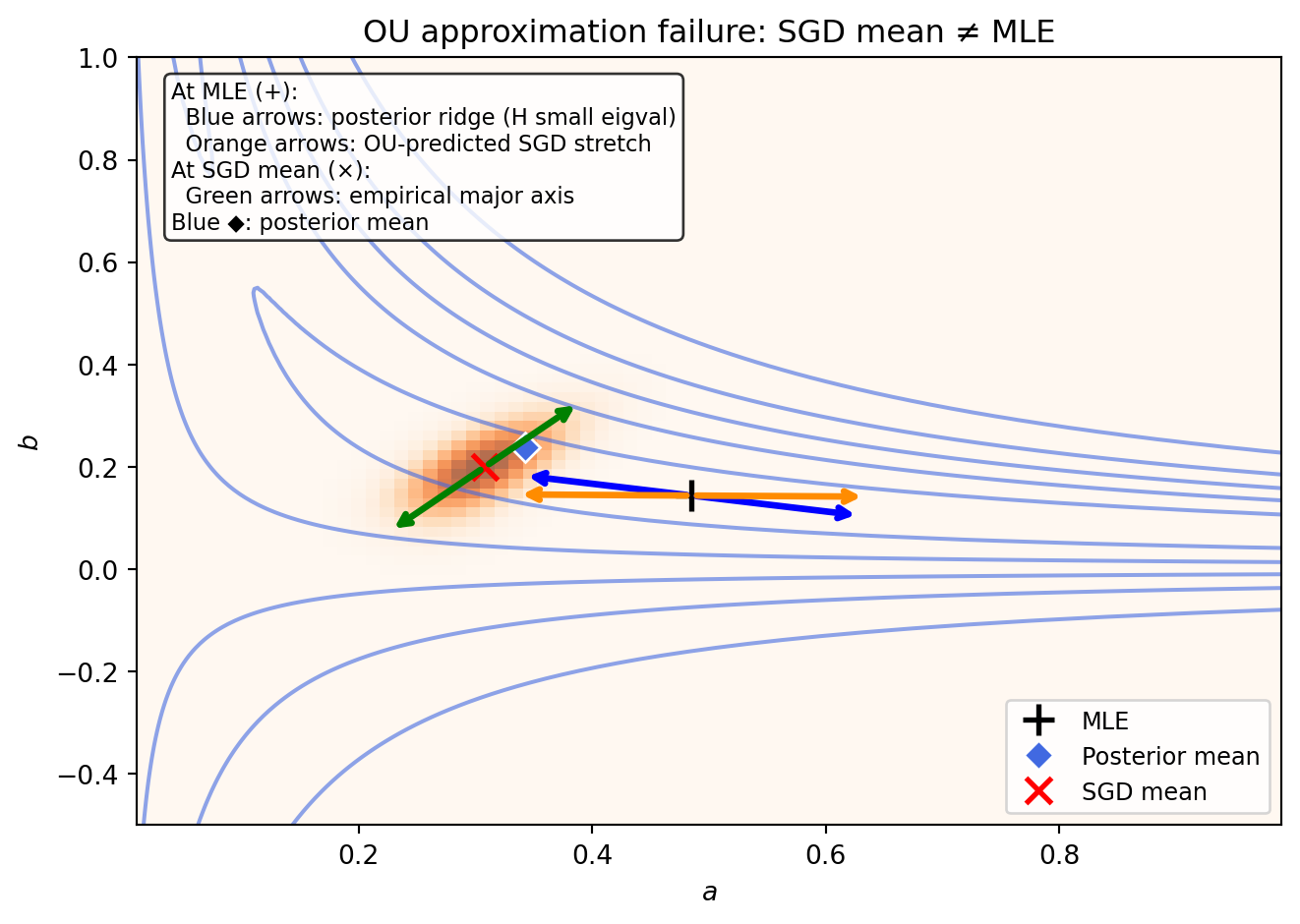
ax.text(0.03, 0.97, 'At MLE (+):\n'
        '  Blue arrows: posterior ridge (H small eigval)\n'
        '  Orange arrows: OU-predicted SGD stretch\n'
        'At SGD mean (×):\n'
        '  Green arrows: empirical major axis\n'
        'Blue ◆: posterior mean',
        transform=ax.transAxes, fontsize=8.5, va='top',
        bbox=dict(boxstyle='round', facecolor='white', alpha=0.8))

ax.legend(loc='lower right', fontsize=9)
ax.set_xlabel('$a$')
ax.set_ylabel('$b$')
ax.set_title('OU approximation failure: SGD mean ≠ MLE')
plt.tight_layout()
plt.show()

MLE:            a* = 0.4852,  b* = 0.1440
SGD traj. mean: a  = 0.3079,  b  = 0.1998
Shift from MLE:      Δa = -0.1773, Δb = 0.0558

Empirical covariance:
  eigenvalues = 0.000515, 0.004525  (ratio 8.8:1)
  major axis angle = 57.1°
OU prediction @ MLE:
  eigenvalues = 0.003952, 0.052390  (ratio 13.3:1)
  major axis angle = 179.2°
OU prediction @ SGD mean:
  eigenvalues = 0.014830, 0.040280  (ratio 2.7:1)
  major axis angle = -152.1°

Posterior mean: a = 0.3423,  b = 0.2384

Figure 3: Comparison of the OU-predicted SGD ellipses with the actual empirical trajectory. The OU theory (evaluated at either the MLE or the SGD mean) fails to predict both the location and shape of the SGD distribution in this singular model.

The results are striking. The SGD trajectory mean is shifted substantially from the MLE — towards smaller \(a\) and larger \(b\), pulled towards the singular set \(a = 0\). The OU theory, which predicts a Gaussian centred at \(w^*\), cannot account for this shift at all. Even if we evaluate \(H\) and \(C\) at the actual SGD mean rather than the MLE, the predicted covariance \(\Sigma = \frac{1}{2B}H^{-1}C\) still fails to match the empirical trajectory covariance: the predicted variances are an order of magnitude too large, and the principal axes point in the wrong direction.

This quantitative failure reinforces the qualitative message: near a singularity, \(H\) and \(C\) vary so rapidly across the region explored by SGD that no single-point linearisation can describe the dynamics. The OU process theory is fundamentally a local approximation, and the singular geometry makes the loss landscape non-quadratic throughout the entire region the SGD trajectory explores.

The Role of Temperature

The effective temperature \(T = \eta / (2B)\) controls the width of the SGD stationary distribution. Let us visualize this systematically for both models.

alphas = [0.1, 0.5, 1.0, 2.0, 5.0]
fig, axes = plt.subplots(2, len(alphas), figsize=(16, 7), 
                          gridspec_kw={'hspace': 0.35, 'wspace': 0.15})

batch_size = 10

# Model 1 (top row)
for j, alpha in enumerate(alphas):
    ax = axes[0, j]
    eta = 2.0 * batch_size * alpha / n
    traj = cached_sgd(sgd_model1, X, eta, batch_size, n_steps=200000, burn_in=5000, seed=42)
    
    hist, _, _ = np.histogram2d(traj[:, 0], traj[:, 1], bins=80,
                                 range=[[-0.6, 0.6], [0.5, 1.5]])
    hist = gaussian_filter(hist.T, sigma=1.5)
    hist /= np.max(hist)
    
    ax.imshow(hist, origin='lower', extent=[-0.6, 0.6, 0.5, 1.5],
              aspect='auto', cmap='Oranges', alpha=0.85)
    ax.contour(A_grid, Sigma_grid, posterior / np.max(posterior),
               levels=[0.1, 0.3, 0.5, 0.7, 0.9],
               colors='royalblue', linewidths=1.0)
    ax.plot(0, 1, 'w+', markersize=8, markeredgewidth=2)
    ax.set_title(rf'$\alpha = {alpha}$', fontsize=10)
    if j == 0:
        ax.set_ylabel(r'Regular: $\sigma$')
    else:
        ax.set_yticklabels([])
    ax.set_xticklabels([])

# Model 2 (bottom row)
for j, alpha in enumerate(alphas):
    ax = axes[1, j]
    eta = 2.0 * batch_size * alpha / n2
    traj = cached_sgd(sgd_model2, X2, eta, batch_size, n_steps=300000, burn_in=10000, seed=42)
    
    hist, _, _ = np.histogram2d(traj[:, 0], traj[:, 1], bins=80,
                                 range=[[0.01, 0.99], [-0.5, 1.0]])
    hist = gaussian_filter(hist.T, sigma=1.5)
    hist /= np.max(hist)
    
    ax.imshow(hist, origin='lower', extent=[0.01, 0.99, -0.5, 1.0],
              aspect='auto', cmap='Oranges', alpha=0.85)
    ax.contour(A_grid2, B_grid2, posterior2 / np.max(posterior2),
               levels=[0.1, 0.3, 0.5, 0.7, 0.9],
               colors='royalblue', linewidths=1.0)
    ax.plot(0.5, 0.3, 'w+', markersize=8, markeredgewidth=2)
    ax.set_xlabel('$a$')
    if j == 0:
        ax.set_ylabel('Singular: $b$')
    else:
        ax.set_yticklabels([])

fig.suptitle(r'SGD Temperature Sweep: $T = \alpha / n$  (orange = SGD, blue contours = posterior)',
             fontsize=13, y=1.02)
plt.show()

Figure 4: Effect of temperature on the SGD stationary distribution for both models. Each column corresponds to a different temperature factor \(\alpha\), where \(T = \alpha/n\). At \(\alpha = 1\) (the Bayesian temperature), the SGD distribution should best approximate the posterior.

Quantitative Comparison: Marginal Distributions

To go beyond visual comparison, let us overlay the one-dimensional marginal distributions of the SGD trajectory against the exact posterior marginals.

fig, axes = plt.subplots(2, 2, figsize=(12, 8))

# --- Model 1 marginals ---
batch_size = 10
eta = 2.0 * batch_size / n
traj1 = cached_sgd(sgd_model1, X, eta, batch_size, n_steps=300000, burn_in=5000, seed=42)

# Marginal over a
da = a_grid[1] - a_grid[0]
dsig = sigma_grid[1] - sigma_grid[0]
post1_a = posterior.sum(axis=0) * dsig
post1_a /= post1_a.sum() * da

axes[0, 0].hist(traj1[:, 0], bins=100, density=True, alpha=0.6, color='orange', label='SGD')
axes[0, 0].plot(a_grid, post1_a, 'royalblue', lw=2, label='Posterior')
axes[0, 0].set_xlabel('$a$')
axes[0, 0].set_ylabel('Density')
axes[0, 0].set_title('Regular Model: marginal of $a$')
axes[0, 0].legend()

# Marginal over sigma
post1_sig = posterior.sum(axis=1) * da
post1_sig /= post1_sig.sum() * dsig

axes[0, 1].hist(traj1[:, 1], bins=100, density=True, alpha=0.6, color='orange', label='SGD')
axes[0, 1].plot(sigma_grid, post1_sig, 'royalblue', lw=2, label='Posterior')
axes[0, 1].set_xlabel(r'$\sigma$')
axes[0, 1].set_title(r'Regular Model: marginal of $\sigma$')
axes[0, 1].legend()

# --- Model 2 marginals ---
eta2 = 2.0 * batch_size / n2
traj2 = cached_sgd(sgd_model2, X2, eta2, batch_size, n_steps=400000, burn_in=10000, seed=42)

da2 = a_grid2[1] - a_grid2[0]
db2 = b_grid2[1] - b_grid2[0]

post2_a = posterior2.sum(axis=0) * db2
post2_a /= post2_a.sum() * da2

axes[1, 0].hist(traj2[:, 0], bins=100, density=True, alpha=0.6, color='orange', label='SGD')
axes[1, 0].plot(a_grid2, post2_a, 'royalblue', lw=2, label='Posterior')
axes[1, 0].set_xlabel('$a$')
axes[1, 0].set_ylabel('Density')
axes[1, 0].set_title('Singular Model: marginal of $a$')
axes[1, 0].legend()

post2_b = posterior2.sum(axis=1) * da2
post2_b /= post2_b.sum() * db2

axes[1, 1].hist(traj2[:, 1], bins=100, density=True, alpha=0.6, color='orange', label='SGD')
axes[1, 1].plot(b_grid2, post2_b, 'royalblue', lw=2, label='Posterior')
axes[1, 1].set_xlabel('$b$')
axes[1, 1].set_title('Singular Model: marginal of $b$')
axes[1, 1].legend()

plt.tight_layout()
plt.show()

Figure 5: Marginal distributions of SGD trajectory (orange histograms) vs exact posterior marginals (blue curves) at the Bayesian-optimal temperature, for both models.

Summary

Aspect	Regular Model	Singular Model
Posterior shape	Gaussian (Bernstein–von Mises)	Non-Gaussian, along singular manifold
OU process approximation	Excellent	Poor
SGD ≈ posterior at \(T = 1/n\)?	Yes	Only qualitative agreement
Temperature control	Precise via \(\eta/(2B)\)	Approximate only

Key takeaways:

1. SGD with constant learning rate is an approximate Bayesian sampler. The effective temperature is \(T = \eta/(2B)\), and setting \(\eta = 2B/n\) makes SGD sample from an approximation of the posterior.

2. For regular models, the approximation is excellent. The posterior is Gaussian, the OU process theory applies, and the SGD distribution faithfully reproduces it.

3. For singular models, the approximation degrades. The non-Gaussian posterior geometry—precisely the kind studied by Watanabe’s Singular Learning Theory—cannot be captured by the quadratic (OU process) approximation. The SGD trajectory still explores regions of high posterior density, but its distribution is systematically different from the true posterior.

4. This connects optimisation to Bayesian inference. Even practitioners who “just do SGD” are implicitly performing approximate Bayesian inference, with the learning rate and batch size jointly determining the effective prior strength.