Regular and Singular Models

This document reproduces Figures 1.2 to 1.5 from Sumio Watanabe’s Mathematical Theory of Bayesian Statistics, demonstrating the fundamental differences between regular and singular statistical models.

Overview

In Bayesian statistics, we observe how the posterior distribution behaves as the sample size \(n\) increases.

• Regular Models: Provide a one-to-one mapping from parameters to probability distributions with a strictly positive-definite Fisher information matrix. By the Bernstein-von Mises theorem, the posterior distribution asymptotically approaches a normal distribution, regardless of the specific sample realization.
• Singular Models: Feature unidentifiable parameters or a degenerate Fisher information matrix. The posterior distribution does not converge to a normal distribution, regardless of sample size, and its shape varies wildly depending on the specific realization of the data.

We generate multiple datasets for different sample sizes to visualize these properties.

Model 1: A Regular Statistical Model

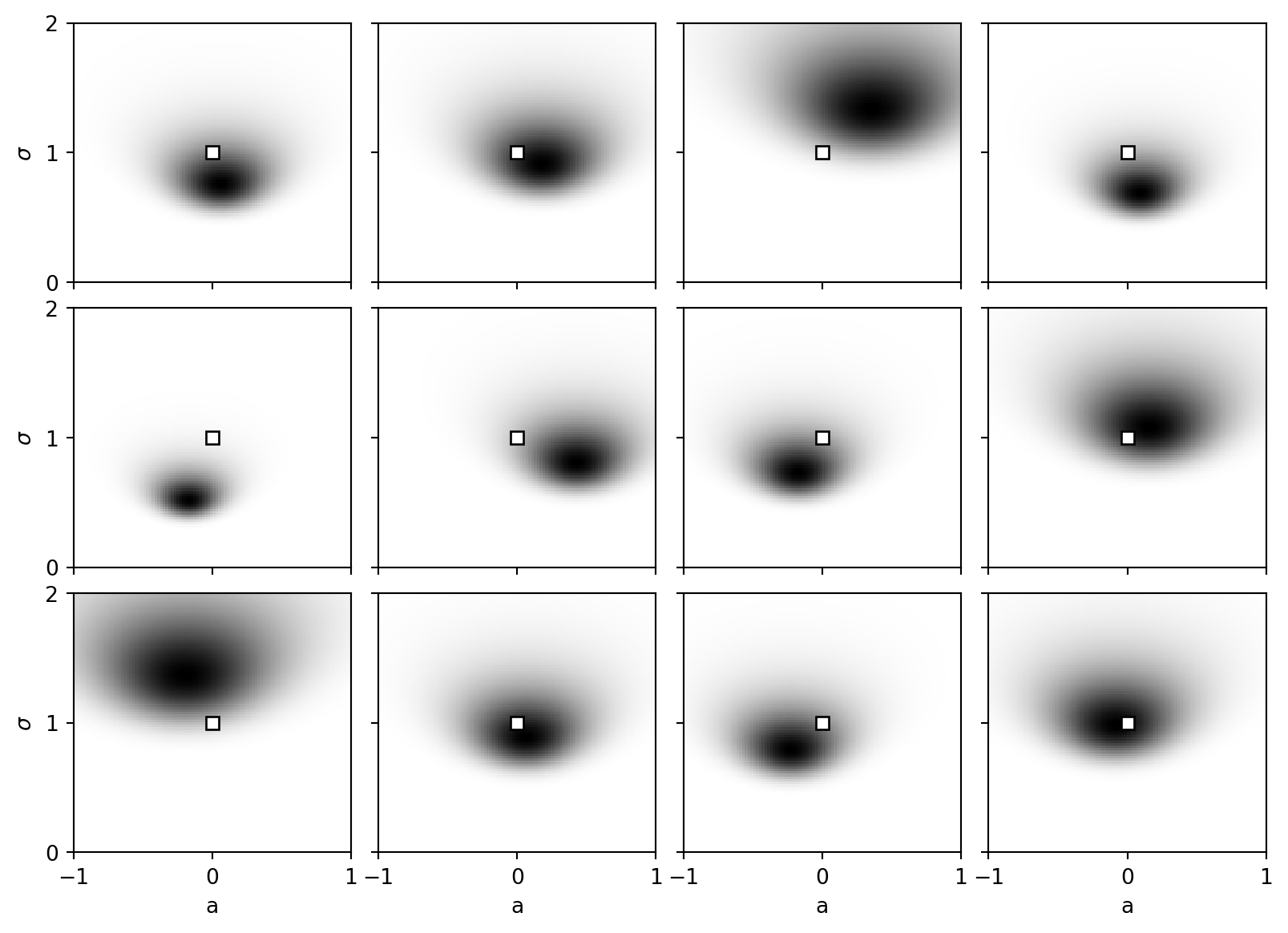
In our first model (Eq. 1.11), the data is drawn from a standard normal distribution \(\mathcal{N}(0, 1)\). We model this with a normal distribution with an unknown mean \(a\) and standard deviation \(\sigma\). \[p(x \mid a, \sigma) = \frac{1}{\sqrt{2\pi\sigma^2}} \exp\left(-\frac{(x - a)^2}{2\sigma^2}\right)\] The true parameters are \(a = 0\) and \(\sigma = 1\). The Fisher Information Matrix at the true parameters is positive definite, making this a regular model.

def generate_data_model1(n, num_datasets=12, seed=42):
    np.random.seed(seed)
    return np.random.normal(loc=0.0, scale=1.0, size=(num_datasets, n))

def posterior_model1(x, a_range, sigma_range):
    A, Sigma = np.meshgrid(a_range, sigma_range)
    x_reshaped = x.reshape(-1, 1, 1)
    log_likelihood_all = -0.5 * np.log(2 * np.pi * Sigma**2) - 0.5 * ((x_reshaped - A) / Sigma)**2
    log_likelihood = np.sum(log_likelihood_all, axis=0)
    
    log_posterior = log_likelihood - np.max(log_likelihood)
    posterior = np.exp(log_posterior)
    posterior /= np.sum(posterior)
    return A, Sigma, posterior

def plot_model1(n, num_datasets=12):
    data = generate_data_model1(n, num_datasets, seed=n)
    a_vals = np.linspace(-1, 1, 100)
    sigma_vals = np.linspace(0.01, 2.0, 100)
    
    fig, axes = plt.subplots(3, 4, figsize=(10, 7), sharex=True, sharey=True)
    fig.subplots_adjust(wspace=0.1, hspace=0.1)
    
    for i in range(num_datasets):
        ax = axes[i // 4, i % 4]
        A, Sigma, post = posterior_model1(data[i], a_vals, sigma_vals)
        ax.imshow(post, origin='lower', extent=[-1, 1, 0.01, 2.0], aspect='auto', cmap='gray_r')
        ax.plot(0, 1, 'ws', markersize=6, markeredgecolor='k')
        
        ax.set_xticks([-1, 0, 1])
        ax.set_yticks([0, 1, 2])
        if i // 4 == 2:
            ax.set_xlabel('a')
        if i % 4 == 0:
            ax.set_ylabel(r'$\sigma$')
            
    plt.show()

Reproducing Figure 1.2 (\(n = 10\))

Here we visualize the posterior distribution for 12 different generated datasets, each with \(n=10\) observations. The true parameter value \((a=0, \sigma=1)\) is indicated by the white square. With a small sample size, the posteriors are broad and slightly irregular, heavily influenced by the specific data samples.

plot_model1(10)

Reproducing Figure 1.3 (\(n = 50\))

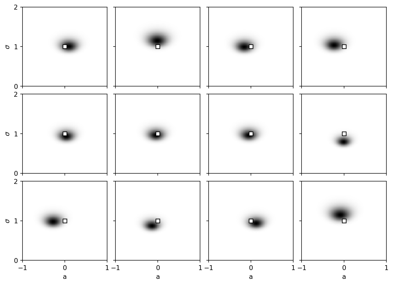
When we increase the sample size to \(n=50\), two things happen: 1. The posterior probability mass tightly concentrates around the true parameter \((0, 1)\). 2. The shape of the posterior takes on a consistent, isotropic ‘blob’ (a Gaussian profile), independent of the precise sampling variations. This is a hallmark of regular models.

plot_model1(50)

Model 2: A Singular Statistical Model

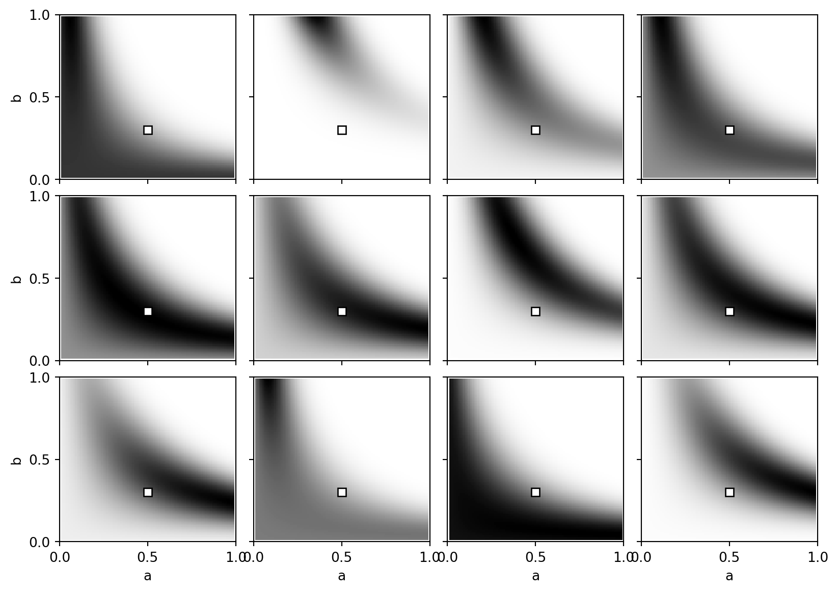
Our second model (Eq. 1.12) fits a two-component Gaussian mixture to data. The data is generated as a 50/50 mix of \(\mathcal{N}(0, 1)\) and \(\mathcal{N}(0.3, 1)\). Our model tries to learn the mixture proportions and the mean of the second component: \[p(x \mid a, b) = (1 - a) \mathcal{N}(x \mid 0, 1) + a \mathcal{N}(x \mid b, 1)\]

The true distribution represents \(a = 0.5\) and \(b = 0.3\). This model is singular. The mapping from parameters to distribution is not identifiable or one-to-one, and the Fisher information matrix rank decreases at these singularities. Consequently, standard statistical theory (like AIC or the Laplace approximation) fails because the posterior is not normally distributed.

def generate_data_model2(n, num_datasets=12, seed=42):
    np.random.seed(seed)
    data = []
    for _ in range(num_datasets):
        components = np.random.choice([0, 1], size=n, p=[0.5, 0.5])
        means = np.where(components == 0, 0.0, 0.3)
        sample = np.random.normal(loc=means, scale=1.0)
        data.append(sample)
    return np.array(data)

def posterior_model2(x, a_range, b_range):
    A, B = np.meshgrid(a_range, b_range)
    x_reshaped = x.reshape(-1, 1, 1)
    p1 = np.exp(-0.5 * x_reshaped**2) / np.sqrt(2 * np.pi)
    p2 = np.exp(-0.5 * (x_reshaped - B)**2) / np.sqrt(2 * np.pi)
    px = (1 - A) * p1 + A * p2
    log_likelihood = np.sum(np.log(px + 1e-15), axis=0)
        
    log_posterior = log_likelihood - np.max(log_likelihood)
    posterior = np.exp(log_posterior)
    posterior /= np.sum(posterior)
    return A, B, posterior

def plot_model2(n, num_datasets=12):
    data = generate_data_model2(n, num_datasets, seed=n)
    a_vals = np.linspace(0.01, 0.99, 100)
    b_vals = np.linspace(0.01, 0.99, 100)
    
    fig, axes = plt.subplots(3, 4, figsize=(10, 7), sharex=True, sharey=True)
    fig.subplots_adjust(wspace=0.1, hspace=0.1)
    
    for i in range(num_datasets):
        ax = axes[i // 4, i % 4]
        A, B, post = posterior_model2(data[i], a_vals, b_vals)
        ax.imshow(post, origin='lower', extent=[0.01, 0.99, 0.01, 0.99], aspect='auto', cmap='gray_r')
        ax.plot(0.5, 0.3, 'ws', markersize=6, markeredgecolor='k')
        
        ax.set_xticks([0, 0.5, 1])
        ax.set_yticks([0, 0.5, 1])
        if i // 4 == 2:
            ax.set_xlabel('a')
        if i % 4 == 0:
            ax.set_ylabel('b')
            
    plt.show()

Reproducing Figure 1.4 (\(n = 100\))

Although \(n=100\) is a relatively large sample size, the posterior surfaces (for 12 independent samples) display chaotic geometries. Rather than single circular peaks, the distributions exhibit long, extended ridges and multiple local maxima.

plot_model2(100)

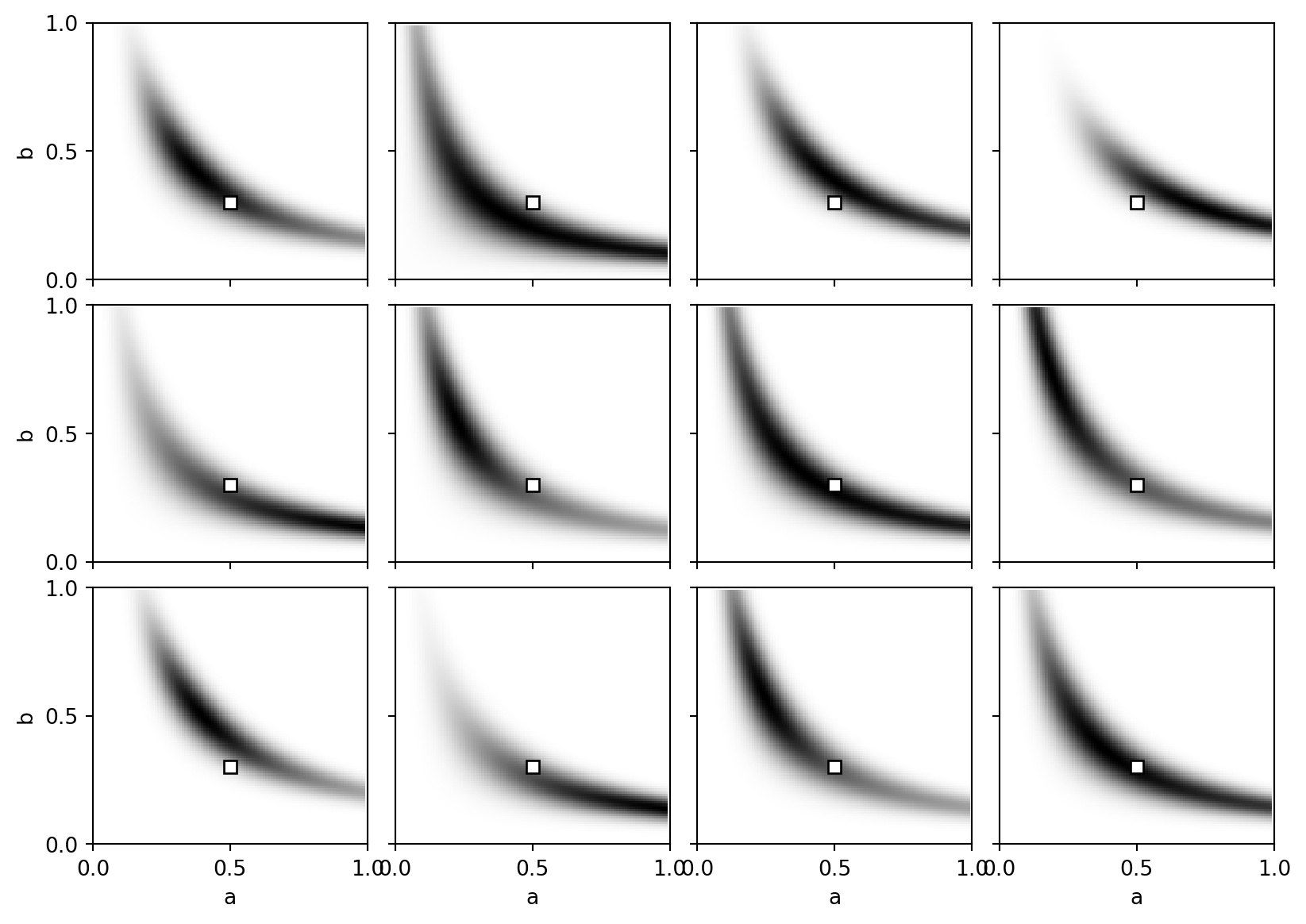
Reproducing Figure 1.5 (\(n = 1000\))

Even at \(n=1000\) (a 10-fold increase), the posterior fails to converge to a neatly shaped Gaussian point cloud. The shape of the distribution remains idiosyncratic, fundamentally dependent on the exact sample drawn. The unidentifiability limits parameter collapse in specific directions—demonstrated by the ‘stretched’ variance seen uniquely across the twelve trials. This highlights the inherent flaw in trying to approximate singular posterior distributions with single-point estimates (e.g. maximum likelihood) or simple quadratics (like the Laplace approximation).

plot_model2(1000)

We will use this example to illustrate the concepts of singular learning theory in SLT Gaussian Mixture.