3 Roots 1

Success is the sum of small efforts, repeated day in and day out.
–Zeno of Elea

3.1 Introduction to Numerical Root Finding

In this chapter and the next we want to solve equations using a computer. Because it takes time to get used to doing numerical calculations we have split this material over two weeks.¹ In this chapter we will cover the bisection method and fixed point iteration. In the next chapter we will cover the Newton-Raphson and secant methods.

The goal of equation solving is to find the value of the independent variable which makes the equation true. These are the sorts of equations that you learned to solve at school. For a very simple example, solve for $x$ if $x+5 = 2x- 3$. Or, for another example, the equation $x^2+x=2x - 7$ is an equation that could be solved with the quadratic formula. The equation $\sin(x) = \frac{\sqrt{2}}{2}$ is an equation which can be solved using some knowledge of trigonometry. The topic of Numerical Root Finding really boils down to approximating the solutions to equations without using all of the by-hand techniques that you learned in high school. The down side to everything that we are about to do is that our answers are only ever going to be approximations.

The fact that we will only ever get approximate answers begs the question: why would we want to do numerical algebra if by-hand techniques exist? The answers are relatively simple:

Most equations do not lend themselves to by-hand solutions. The reason you may not have noticed that is that we tend to show you only nice equations that arise in often very simplified situations. When equations arise naturally they are often not nice.
By-hand algebra is often very challenging, quite time consuming, and error prone. You will find that the numerical techniques are quite elegant, work very quickly, and require very little overhead to actually implement and verify.

Let us first take a look at equations in a more abstract way. Consider the equation $\ell(x) = r(x)$ where $\ell(x)$ and $r(x)$ stand for left-hand and right-hand expressions respectively. To begin solving this equation we can first rewrite it by subtracting the right-hand side from the left to get \[\begin{equation} \ell(x) - r(x) = 0. \end{equation}\] Hence, we can define a function $f(x)$ as $f(x)=\ell(x)-r(x)$ and observe that every equation can be written as: \[\begin{equation} \text{ Find } x \text{ such that } f(x) = 0. \end{equation}\] This gives us a common language for which to frame all of our numerical algorithms. An $x$ where $f(x)=0$ is called a root of $f$ and thus we have seen that solving an equation is always a root finding problem.

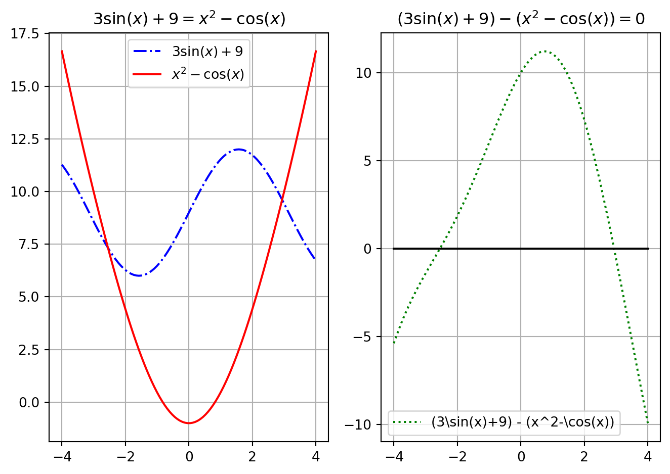
For example, if we want to solve the equation $3\sin(x) + 9 = x^2 - \cos(x)$ then this is the same as solving $(3\sin(x) + 9 ) - (x^2 - \cos(x)) = 0$. We illustrate this idea in Figure 3.1. You should pause and notice that there is no way that you are going to apply by-hand techniques from algebra to solve this equation … an approximate answer is pretty much our only hope.

Code

import numpy as np 
import matplotlib.pyplot as plt
x = np.linspace(-4,4, 100) 
l = 3 * np.sin(x) + 9
r = x**2 - np.cos(x)

fig, axes = plt.subplots(nrows = 1, ncols = 2)

axes[0].plot(x, l, 'b-.', label=r"$3\sin(x)+9$")
axes[0].plot(x, r, 'r-', label=r"$x^2-\cos(x)$")
axes[0].grid()
axes[0].legend()
axes[0].set_title(r"$3\sin(x)+9 = x^2-\cos(x)$")

axes[1].plot(x, l-r, 'g:', label=r"(3\sin(x)+9) - (x^2-\cos(x))")
axes[1].plot(x, np.zeros(100), 'k-')
axes[1].grid()
axes[1].legend()
axes[1].set_title(r"$(3\sin(x)+9) - (x^2-\cos(x))=0$")

fig.tight_layout()
plt.show()

Figure 3.1: Two ways to visualise the same root finding problem

On the left-hand side of Figure 3.1 we see the solutions as the intersections of the graph of $3\sin(x) + 9$ with the graph of $x^2 - \cos(x)$, and on the right-hand side we see the solutions as the intersections of the graph of $\left( 3\sin(x)+9 \right) - \left( x^2 - \cos(x) \right)$ with the $x$ axis. From either plot we can read off the approximate solutions: $x_1 \approx -2.55$ and $x_2 \approx 2.88$. Figure 3.1 should demonstrate what we mean when we say that solving equations of the form $\ell(x) = r(x)$ will give the same answer as finding the roots of $f(x) = \ell(x)-r(x)$.

We now have one way to view every equation-solving problem. As we will see in this chapter, if $f(x)$ has certain properties then different numerical techniques for solving the equation will apply – and some will be much faster and more accurate than others. In the following sections you will develop several different techniques for solving equations of the form $f(x) = 0$. You will start with the simplest techniques to implement and then move to the more powerful techniques that use some ideas from Calculus to understand and analyse. Throughout this chapter you will also work to quantify the amount of error that one makes when using these techniques.

This chapter is split over two weeks. In the first week we will cover the bisection method and fixed point iteration. In the second week we will cover the Newton-Raphson and secant methods.

3.2 The Bisection Method

3.2.1 Intuition

This section contains several discussion exercises to get you thinking about the bisection method. You may not have anyone around to discuss with, in which case you should just discuss the questions with yourself, i.e., think through the questions. When you next meet with your group you can then discuss them with your peers.

Exercise 3.1 💬 A friend tells you that she is thinking of a number between 1 and 100. She will allow you multiple guesses with some feedback for where the mystery number falls. How do you systematically go about guessing the mystery number? Is there an optimal strategy?

For example, the conversation might go like this.

Sally: I am thinking of a number between 1 and 100.
Joe: Is it 35?
Sally: No, 35 is too low.
Joe: Is it 99?
Sally: No, 99 is too high.
…

Exercise 3.2 💬 Imagine that Sally likes to formulate her answer not in the form “$x$ is too small” or “$x$ is too large” but in the form “$f(x)$ is positive” or “$f(x)$ is negative”. If she uses $f(x) = x-x_0$, where $x_0$ is Sally’s chosen number then her new answers contain exactly the same information as her previous answers? Can you now explain how Sally’s game is a root finding game?

Exercise 3.3 💬 Now go and play the game with other functions $f(x)$. Choose someone from your group to be Sally and someone else to be Joe. Sally can choose a continuous function and Joe needs to guess its root. Does your strategy still allow Joe to find the root of $f(x)$ at least approximately? When should the game stop? Does Sally need to give Joe some extra information to give him a fighting chance?

Exercise 3.4 💬 Was it necessary to say that Sally’s function was continuous? Does your strategy work if the function is not continuous.

Now let us get to the maths. We will start the mathematical discussion with a theorem from Calculus.

Theorem 3.1 (The Intermediate Value Theorem (IVT)) If $f(x)$ is a continuous function on the closed interval $[a,b]$ and $y_*$ lies between $f(a)$ and $f(b)$, then there exists some point $x_* \in [a,b]$ such that $f(x_*) = y_*$.

Exercise 3.5 🖋 Draw a picture of what the intermediate value theorem says graphically.

Exercise 3.6 🖋 If $y_*=0$ the Intermediate Value Theorem gives us important information about solving equations. What does it tell us? Fill in the blanks in the following corollary.

Corollary 3.1 If $f(x)$ is a continuous function on the closed interval $[a,b]$ and if $f(a)$ and $f(b)$ have opposite signs then from the Intermediate Value Theorem we know that there exists some point $x_* \in [a,b]$ such that ____.

The Intermediate Value Theorem (IVT) and its corollary are existence theorems in the sense that they tell us that some point exists. The annoying thing about mathematical existence theorems is that they typically do not tell us how to find the point that is guaranteed to exist. The method that you developed in Exercise 3.1 to Exercise 3.3 gives one possible way to find the root.

In those exercises you likely came up with an algorithm such as this:

Say we know that a continuous function has opposite signs at $x=a$ and $x=b$.
Guess that the root is at the midpoint $m = \frac{a+b}{2}$.
By using the signs of the function, narrow the interval that contains the root to either $[a,m]$ or $[m,b]$.
Repeat until the interval is small enough.

Now we will turn this strategy into computer code that will simply play the game for us. But first we need to pay careful attention to some of the mathematical details.

Exercise 3.7 💬 Where is the Intermediate Value Theorem used in the root-guessing strategy?

Exercise 3.8 💬 Why was it important that the function $f(x)$ is continuous when playing this root-guessing game? Provide a few sketches to demonstrate your answer.

3.2.2 Implementation

Exercise 3.9 (The Bisection Method) 🖋 💬 Goal: We want to solve the equation $f(x) = 0$ for $x$ assuming that the solution $x^*$ is in the interval $[a,b]$. To understand the Bisection Method, have someone in the group sketch a graph of the function $f(x)$ on the interval $[a,b]$. Then together, draw in the steps of the following algorithm:

The Algorithm: We assume that your group member has followed the instructions above and has sketched the graph of a function $f(x)$ that is continuous on the interval $[a,b]$. To make approximations of the solutions to the equation $f(x) = 0$, do the following:

Check to see if $f(a)$ and $f(b)$ have opposite signs. You can do this taking the product of $f(a)$ and $f(b)$.
- If $f(a)$ and $f(b)$ have different signs then what does the IVT tell you?
- If $f(a)$ and $f(b)$ have the same sign then what does the IVT not tell you? What should you do in this case?
- Why does the product of $f(a)$ and $f(b)$ tell us something about the signs of the two numbers?
Compute the midpoint of the closed interval, $m=\frac{a+b}{2}$. Mark the result in your plot so that you can see the value of $f(m)$.
- Will $m$ always be a better guess of the root than $a$ or $b$? Why?
- What should you do here if $f(m)$ is really close to zero?
Compare the signs of $f(a)$ versus $f(m)$ and $f(b)$ versus $f(m)$.
- What do you do if $f(a)$ and $f(m)$ have opposite signs?
- What do you do if $f(m)$ and $f(b)$ have opposite signs?
Choose the new interval $[a,m]$ or $[m,b]$ and repeat steps 2 and 3 for this interval. Stop when the interval containing the root is small enough.

Exercise 3.10 💻 We want to write a Python function for the Bisection Method. Instead of jumping straight into writing the code we should first come up with the structure of the code. It is often helpful to outline the structure as comments in your file. Use the template below and complete the comments. Note how the function starts with a so-called docstring that describes what the function does and explains the function parameters and its return value. This is standard practice and is how the help text is generated that you see when you hover over a function name in your code.

Don’t write the code yet, just complete the comments. I recommend switching off the AI for this exercise because otherwise the AI will keep already suggesting the code while you write the comments.

def bisection(f, a, b, tol=1e-5):
    """
    Find a root of f(x) in the interval [a, b] using the bisection method.

    Parameters:
        f   : function, the function for which we seek a root
        a   : float, left endpoint of the interval
        b   : float, right endpoint of the interval
        tol : float, stopping tolerance

    Returns:
        float: approximate root of f(x)
    """

    # check that a and b have opposite signs
    # if not, return an error and stop

    # calculate the midpoint m = (a+b)/2

    # start a while loop that runs while the interval is 
    # larger than 2 * tol
    
        # if ...
        # elif ...
        # elif ...
        
        # Calculate midpoint of new interval

    # end the while loop
    # return the approximate root

Exercise 3.11 💻 Now use the comments from Exercise 3.10 as structure to complete a Python function for the Bisection Method. Test your Bisection Method code on the following equations. For each equation make a plot of the function on the interval to verify your result.

$x^2 - 2 = 0$ on $x \in [0,2]$
$\sin(x) + x^2 = 2\log(x) + 5$ on $x \in [1,5]$
🎓 $3\sin(x) + 9 = x^2+\cos(x)$ on $x \in [1,5]$

Figure 3.2 shows the bisection method in action on the equation $x^2 - 2 = 0$.

Figure 3.2: An animation of the bisection method in action on the equation $x^2 - 2 = 0$.

3.2.3 Analysis

After we build any root finding algorithm we need to stop and think about how it will perform on new problems. The questions that we typically have for a root-finding algorithm are:

Will the algorithm always converge to a solution?
How fast will the algorithm converge to a solution?
Are there any pitfalls that we should be aware of when using the algorithm?

Exercise 3.12 💬 Discussion:

What must be true in order to use the bisection method?
Does the bisection method work if the Intermediate Value Theorem does not apply? (Hint: what does it mean for the IVT to “not apply?”)
If there is a root of a continuous function $f(x)$ between $x=a$ and $x=b$, will the bisection method always be able to find it? Why / why not?

Next we will focus on a deeper mathematical analysis that will allow us to determine exactly how fast the bisection method actually converges to within a pre-set tolerance. Work through the next problem to develop a formula that tells you exactly how many steps the bisection method needs to take before it gets close enough to the true solution.

Exercise 3.13 🖋 Let $f(x)$ be a continuous function on the interval $[a,b]$ and assume that $f(a) \cdot f(b) <0.$ A recurring theme in Numerical Analysis is to approximate some mathematical thing to within some tolerance. For example, if we want to approximate the solution to the equation $f(x)=0$ to within $\varepsilon$ with the bisection method, we should be able to figure out how many steps it will take to achieve that goal.

Let us say that $a = 3$ and $b = 8$ and $f(a) \cdot f(b) < 0$ for some continuous function $f(x)$. The width of this interval is $5$, so if we guess that the root is $m=(3+8)/2 = 5.5$ then our error is less than $5/2$. In the more general setting, if there is a root of a continuous function in the interval $[a,b]$ then how far off could the midpoint approximation of the root be? In other words, what is the error in using $m=(a+b)/2$ as the approximation of the root?
The bisection method cuts the width of the interval down to a smaller size at every step. As such, the approximation error gets smaller at every step. Fill in the blanks in the following table to see the pattern in how the approximation error changes with each iteration.

Iteration	Width of Interval	Maximal Error
1	$\|b-a\|$	$\frac{\|b-a\|}{2}$
2	$\frac{\|b-a\|}{2}$
3	$\frac{\|b-a\|}{2^2}$
$\vdots$	$\vdots$	$\vdots$
$n$	$\frac{\|b-a\|}{2^{n-1}}$

Now to the key question:
If we want to approximate the solution to the equation $f(x)=0$ to within some tolerance $\varepsilon$ then how many iterations of the bisection method do we need to take?
Hint: Set the $n^{th}$ approximation error from the table equal to $\varepsilon$. What should you solve for from there?

In Exercise 3.13 you actually proved the following theorem.

Theorem 3.2 (Convergence Rate of the Bisection Method) If $f(x)$ is a continuous function with a root in the interval $[a,b]$ and if the bisection method is performed to find the root then:

The error between the actual root and the approximate root will decrease by a factor of 2 at every iteration.
If we want the approximate root found by the bisection method to be within a tolerance of $\varepsilon$ then \[\begin{equation} \frac{|b-a|}{2^{n}} = \varepsilon \end{equation}\] where $n$ is the number of iterations that it takes to achieve that tolerance.

Solving for the number $n$ of iterations we get \[\begin{equation} n = \log_2\left( \frac{|b-a|}{\varepsilon} \right). \end{equation}\]

Rounding the value of $n$ up to the next integer gives the number of iterations necessary to approximate the root to a precision less than $\varepsilon$.

Exercise 3.14 🖋 🎓 Apply what you have learned in Theorem 3.2 to determine how many iterations the bisection method will take to approximate the solution of the equation \[3\sin(x) + 9 = x^2+\cos(x)\] on $x \in [1,5]$ to within a tolerance of $10^{-6}$.

💻 Now create a second version of your Python Bisection Method function that uses a for loop that takes the exact number of steps required to guarantee that the approximation to the root lies within a requested tolerance. This should be in contrast to your first version which likely used a while loop to decide when to stop. Is there an advantage to using one of these version of the Bisection Method over the other?

The final type of analysis that we should do on the bisection method is to make plots of the error between the approximate solution that the bisection method gives you and the exact solution to the equation. This is a bit of a funny thing! Stop and think about this for a second: if you know the exact solution to the equation then why are you solving it numerically in the first place!?!? However, whenever you build an algorithm you need to test it on problems where you actually do know the answer so that you can be somewhat sure that it is not giving you nonsense. Furthermore, analysis like this tells us how fast the algorithm is expected to perform.

From Theorem 3.2 you know that the bisection method cuts the interval in half at every iteration. You proved in Exercise 3.13 that the error given by the bisection method is therefore cut in half at every iteration as well. The following example demonstrate this theorem graphically.

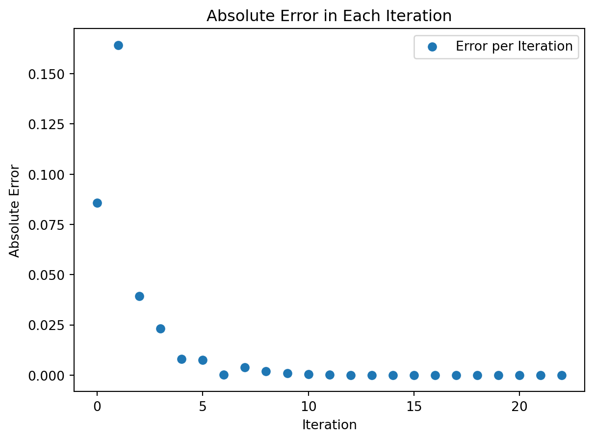
Example 3.1 Let us solve the very simple equation $x^2 - 2 = 0$ for $x$ to get the solution $x = \sqrt{2}$ with the bisection method. Since we know the exact answer we can compare the exact answer to the value of the midpoint given at each iteration and calculate an absolute error: \[\begin{equation} \text{Absolute Error} = | \text{Approximate Solution} - \text{Exact Solution}|. \end{equation}\]

Let us write a Python function that implements the bisection method and collects the absolute errors at each iteration into a list.

def bisection_with_error_tracking(f, x_exact, a, b, tol):
    """
    Implements the bisection method and tracks absolute error at each iteration.
    
    Parameters:
        f (callable): Function for which to find the root
        x_exact (float): The exact root of the function
        a (float): Left endpoint of initial interval
        b (float): Right endpoint of initial interval 
        tol (float): Tolerance for stopping criterion
        
    Returns:
        list: List of absolute errors between approximate and exact solution at each iteration
    """
    errors = []
    while (b - a) / 2.0 > tol:
        midpoint = (a + b) / 2.0
        if f(midpoint) == 0:
            break
        elif f(a) * f(midpoint) < 0:
            b = midpoint
        else:
            a = midpoint
        error = abs(midpoint - x_exact)
        errors.append(error)
    return errors

We can now use this function to see the absolute error at each iteration when solving the equation $x^2-2=0$ with the bisection method.

import numpy as np

def f(x):
    return x**2 - 2

x_exact = np.sqrt(2)

# Using the interval [1, 2] and a tolerance of 1e-7
tolerance = 1e-7
errors = bisection_with_error_tracking(f, x_exact, 1, 2, tolerance)
errors

[np.float64(0.08578643762690485),
 np.float64(0.16421356237309515),
 np.float64(0.039213562373095145),
 np.float64(0.023286437626904855),
 np.float64(0.007963562373095145),
 np.float64(0.0076614376269048545),
 np.float64(0.00015106237309514547),
 np.float64(0.0037551876269048545),
 np.float64(0.0018020626269048545),
 np.float64(0.0008255001269048545),
 np.float64(0.0003372188769048545),
 np.float64(9.307825190485453e-05),
 np.float64(2.8992060595145475e-05),
 np.float64(3.2043095654854525e-05),
 np.float64(1.5255175298545254e-06),
 np.float64(1.3733271532645475e-05),
 np.float64(6.103877001395475e-06),
 np.float64(2.2891797357704746e-06),
 np.float64(3.818311029579746e-07),
 np.float64(5.718432134482754e-07),
 np.float64(9.500605524515038e-08),
 np.float64(1.4341252385641212e-07),
 np.float64(2.4203234305630872e-08)]

Next we write a function to plot the absolute error on the vertical axis and the iteration number on the horizontal axis. We get Figure 3.3. As expected, the absolute error follows an exponentially decreasing trend. Notice that it is not a completely smooth curve since we will have some jumps in the accuracy just due to the fact that sometimes the root will be near the midpoint of the interval and sometimes it will not be.

import matplotlib.pyplot as plt
def plot_errors(errors):
    """
    Plot the absolute errors.
    
    Parameters
        errors (list): List of absolute errors
    """
    # Creating the x values for the plot (iterations) 
    iterations = np.arange(len(errors))

    # Plotting the errors
    plt.scatter(iterations, errors, label='Error per Iteration')
    
    plt.xlabel('Iteration')
    plt.ylabel('Absolute Error') 
    plt.title('Absolute Error in Each Iteration')
    plt.legend()
    plt.show()

plot_errors(errors)

Figure 3.3: The evolution of the absolute error when solving the equation $x^2-2=0$ with the bisection method.

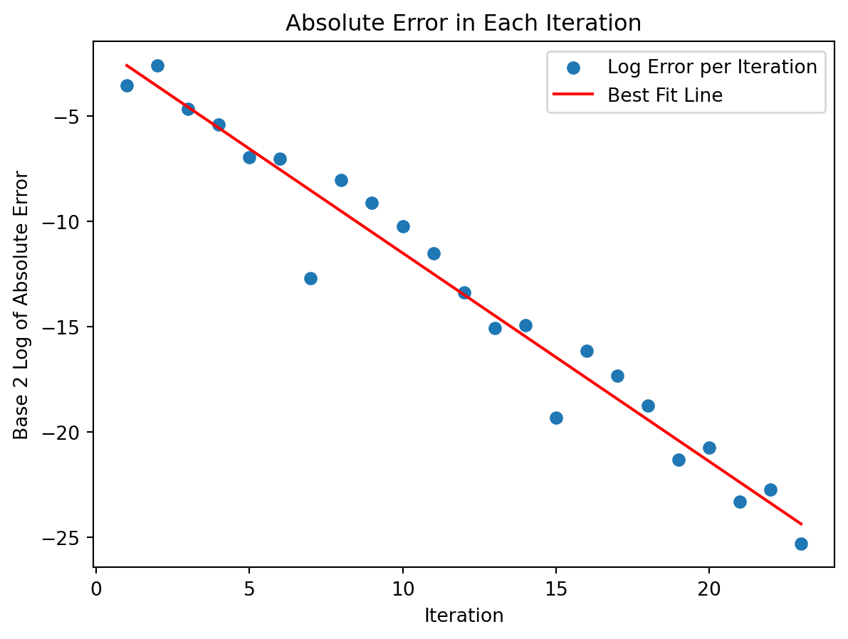
Without Theorem 3.2 it would be rather hard to tell what the exact behaviour is in the exponential plot above. We know from Theorem 3.2 that the error will divide by 2 at every step, so if we instead plot the base-2 logarithm of the absolute error against the iteration number we should see a linear trend as shown in Figure 3.4.

def plot_log_errors(errors):
    """
    Plot the base-2 logarithm of absolute errors and a best fit line.
    
    Parameters:
        errors (list): List of absolute errors
    """
    # Convert errors to base 2 logarithm
    log_errors = np.log2(errors)
    # Creating the x values for the plot (iterations)
    iterations = np.arange(len(log_errors))

    # Plotting the errors
    plt.scatter(iterations, log_errors, label='Log Error per Iteration')

    # Determine slope and intercept of the best-fit straight line
    slope, intercept = np.polyfit(iterations, log_errors, deg=1)
    best_fit_line = slope * iterations + intercept
    # Plot the best-fit line
    plt.plot(iterations, best_fit_line, label='Best Fit Line', color='red')

    plt.xlabel('Iteration')
    plt.ylabel('Base 2 Log of Absolute Error')
    plt.title('Absolute Error in Each Iteration')
    plt.legend()
    plt.show()

plot_log_errors(errors)

Figure 3.4: Iteration number vs the base-2 logarithm of the absolute error. Notice the slope of $-1$ indicating that the error is divided by a factor of 2 at each step of the algorithm.

There will be times later in this course where we will not have a nice theorem like Theorem 3.2 and instead we will need to deduce the relationship from plots like these.

The trend is linear since logarithms and exponential functions are inverses. Hence, applying a logarithm to an exponential will give a linear function.
The slope of the resulting linear function should be $-1$ in this case since we are dividing by a factor of 2 each iteration. You can visually verify that the slope in the plot above follows this trend (the red dashed line in the plot is shown to help you see the slope).

Exercise 3.15 💻 Carefully read and understand all of the details of the previous example and plots. Then create plots similar to that example to solve the equation \[ e^{x-3}+\sqrt{x+6}=4 \] on the interval $x \in [0,5]$ to which the exact solution is $x=3$. You should see the same basic behaviour based on the theorem that you proved in Exercise 3.13. If you do not see the same basic behaviour then something has gone wrong. 💬 Also, the plot will look much more regular than in the previous example. Can you explain why?

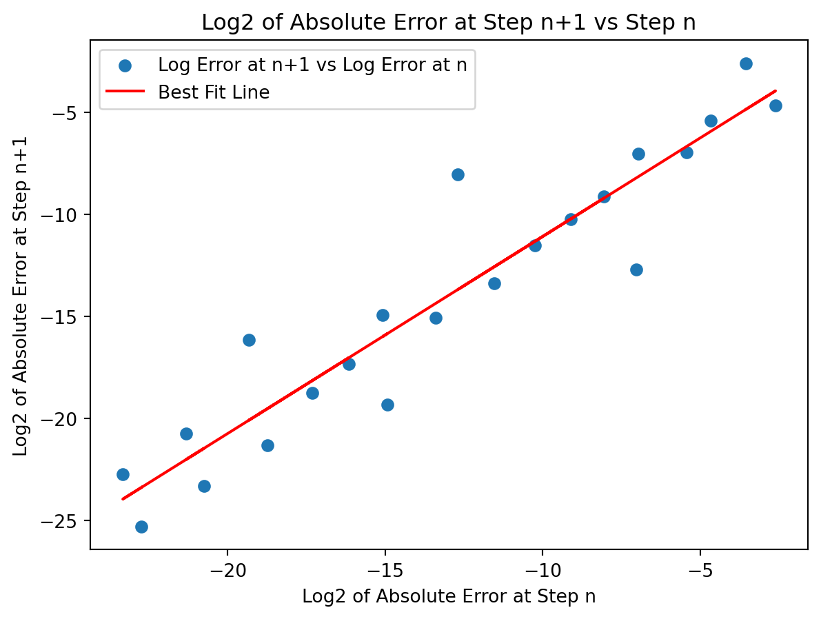
Example 3.2 Another plot that numerical analysts use quite frequently for determining how an algorithm is behaving as it progresses is shown in Figure 3.5. and is defined by the following axes:

The horizontal axis is the absolute error at iteration $n$.
The vertical axis is the absolute error at iteration $n+1$.

def plot_error_progression(errors):
    # Calculating the log2 of the absolute error at step n and n+1
    log_errors = np.log2(errors)
    log_errors_n = log_errors[:-1]  # log errors at step n (excluding the last one)
    log_errors_n_plus_1 = log_errors[1:]  # log errors at step n+1 (excluding the first one)

    # Plotting log_errors_n+1 vs log_errors_n
    plt.scatter(log_errors_n, log_errors_n_plus_1, label='Log Error at n+1 vs Log Error at n')

    # Fitting a straight line to the data points
    slope, intercept = np.polyfit(log_errors_n, log_errors_n_plus_1, deg=1)
    best_fit_line = slope * log_errors_n + intercept
    plt.plot(log_errors_n, best_fit_line, color='red', label='Best Fit Line')

    # Setting up the plot
    plt.xlabel('Log2 of Absolute Error at Step n')
    plt.ylabel('Log2 of Absolute Error at Step n+1')
    plt.title('Log2 of Absolute Error at Step n+1 vs Step n')
    plt.legend()
    plt.show()

plot_error_progression(errors)

Figure 3.5: The base-2 logarithm of the absolute error at iteration $n$ vs the base-2 logarithm of the absolute error at iteration $n+1$.

This type of plot takes a bit of explaining the first time you see it. Each point in the plot corresponds to an iteration of the algorithm. The x-coordinate of each point is the base-2 logarithm of the absolute error at step $n$ and the y-coordinate is the base-2 logarithm of the absolute error at step $n+1$. The initial interations are on the right-hand side of the plot where the error is the largest (this will be where the algorithm starts). As the iterations progress and the error decreases the points move to the left-hand side of the plot. Examining the slope of the trend line in this plot shows how we expect the error to progress from step to step. The slope appears to be about $1$ in Figure 3.5 and the intercept appears to be about $-1$. In this case we used a base-2 logarithm for each axis so we have just empirically shown that \[\begin{equation} \log_2(\text{absolute error at step $n+1$}) \approx 1\cdot \log_2(\text{absolute error at step $n$}) -1. \end{equation}\] Exponentiating both sides we see that this linear relationship turns into (You should stop now and do this algebra.) Rearranging a bit more we get \[\begin{equation} (\text{absolute error at step $n+1$}) = \frac{1}{2}(\text{absolute error at step $n$}), \end{equation}\] exactly as expected!! Pause and ponder this result for a second – we just empirically verified the convergence rate for the bisection method just by examining Figure 3.5. That’s what makes these types of plots so useful!

Exercise 3.16 💻 Reproduce plots like that in the previous example but for the equation that you used in Exercise 3.15. Again check that the plots have the expected shape.

3.3 Fixed Point Iteration

We will now investigate a different problem that is closely related to root finding: the fixed point problem. Given a function $g$ (of one real argument with real values), we look for a number $p$ such that \[ g(p)=p. \] This $p$ is called a fixed point of $g$.

Any root finding problem $f(x)=0$ can be reformulated as a fixed point problem, and this can be done in many (in fact, infinitely many) ways. For example, given $f$, we can define $g(x):=f(x) + x$; then \[ f(x) = 0 \quad \Leftrightarrow\quad g(x)=x. \] Just as well, we could set $g(x):=\lambda f(x) + x$ with any $\lambda\in{\mathbb R}\backslash\{0\}$, and there are many other possibilities.

The heuristic idea for approximating a fixed point of a function $g$ is quite simple. We take an initial approximation $x_{0}$ and calculate subsequent approximations using the formula \[ x_{n}:=g(x_{n-1}). \] A graphical representation of this sequence when $g = \cos$ and $x_0=2$ is shown in Figure 3.6.

To view the animation, click on the play button below the plot.

Figure 3.6: Fixed point iteration $x_{n} = \cos(x_{n-1})$.

Exercise 3.17 💬 The plot that emerges in Figure 3.6 is known as a cobweb diagram, for obvious reason. Explain to others in your group what is happening in the animation in Figure 3.6 and how that animation is related to the fixed point iteration $x_{n} = \cos(x_{n-1})$.

Exercise 3.18 🎓 The animation in Figure 3.6 is a graphical representation of the fixed point iteration $x_{n} = \cos(x_{n-1})$. Use Python to calculate the first 10 iterations of this sequence with $x_0=0.2$. Use that to get an estimate of the solution to the equation $\cos(x)-x=0$.

Why is the sequence $(x_n)$ expected to approximate a fixed point? Suppose for a moment that the sequence $(x_n)$ converges to some number $p$, and that $g$ is continuous. Then \[ p=\lim_{n\to\infty}x_{n}=\lim_{n\to\infty}g(x_{n-1})= g\left(\lim_{n\to\infty}x_{n-1}\right)=g(p). \tag{3.1}\] Thus, if the sequence converges, then it converges to a fixed point. However, this resolves the problem only partially. One would like to know:

Under what conditions does the sequence $(x_n)$ converge?
How fast is the convergence, i.e., can one obtain an estimate for the approximation error?

So there is much for you to investigate!

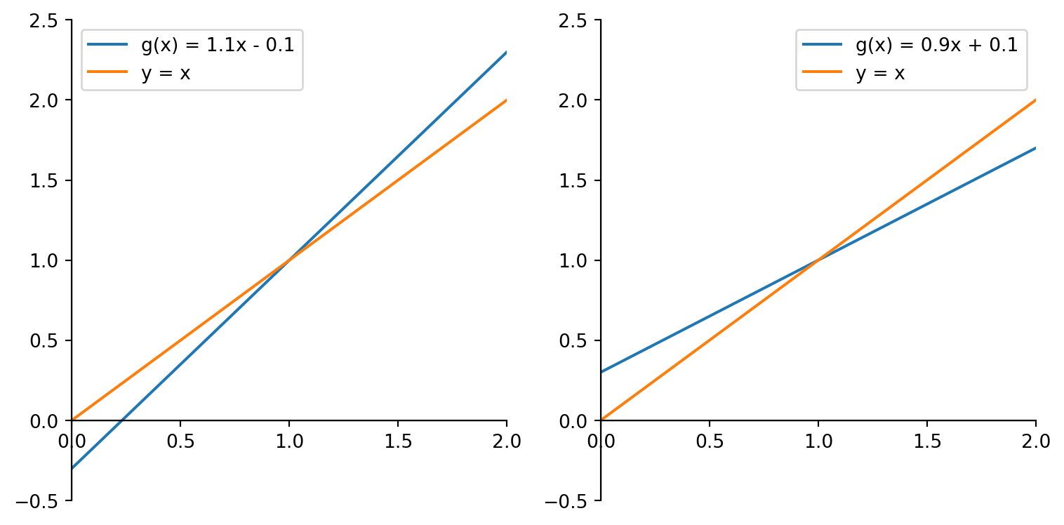
Exercise 3.19 🖋 Copy the two plots in Figure 3.7 to a piece of paper and draw the first few iterations of the fixed point iteration $x_{n} = g(x_{n-1})$ on each of them. In the first plot start with $x_0=0.2$ and in the second plot start with $x_0=1.5$ and in the second plot start with $x=0.9$ What do you observe about the convergence of the sequence in each case?

Figure 3.7: Two plots for practicing your cobweb skills.

Can you make some conjectures about when the sequence $(x_n)$ will converge to a fixed point and when it will not?

Exercise 3.20 🖋 Make similar plots as in the previous exercise but with different slopes of the blue line. Can you make some conjectures about how the speed of convergence is related to the slope of the blue line?

Now see if your observations are in agreement with the following theorem:

Theorem 3.3 (Fixed Point Theorem) Suppose that $g:[a,b]\to [a,b]$ is differentiable, and that there exists $0<k<1$ such that \[ \lvert g^{\prime}(x)\rvert\leq k\quad \text{for all }x \in (a,b). \tag{3.2}\] Then, $g$ has a unique fixed point $p\in [a,b]$; and for any choice of $x_0 \in [a,b]$, the sequence defined by \[ x_{n}:=g(x_{n-1}) \quad \text{for all }n\ge1 \tag{3.3}\] converges to $p$. The following estimate holds: \[ \lvert p- x_{n}\rvert \leq k^n \lvert p-x_{0}\rvert \quad \text{for all }n\geq1. \tag{3.4}\]

Proof. The proof of this theorem is not difficult, but you can skip it and go directly to Exercise 3.21 if you feel that the theorem makes intuitive sense and you are not interested in proofs.

We first show that $g$ has a fixed point $p$ in $[a,b]$. If $g(a)=a$ or $g(b)=b$ then $g$ has a fixed point at an endpoint. If not, then it must be true that $g(a)>a$ and $g(b)<b$. This means that the function $h(x):=g(x)-x$ satisfies \[ \begin{aligned} h(a) &= g(a)-a>0, & h(b)&=g(b)-b<0 \end{aligned} \] and since $h$ is continuous on $[a,b]$ the Intermediate Value Theorem guarantees the existence of $p\in(a,b)$ for which $h(p)=0$, equivalently $g(p)=p$, so that $p$ is a fixed point of $g$.

To show that the fixed point is unique, suppose that $q\neq p$ is a fixed point of $g$ in $[a,b]$. The Mean Value Theorem implies the existence of a number $\xi\in(\min\{p,q\},\max\{p,q\})\in(a,b)$ such that \[ \frac{g(p)-g(q)}{p-q}=g'(\xi). \] Then \[ \lvert p - q\rvert = \lvert g(p)-g(q) \rvert = \lvert (p-q)g'(\xi) \rvert = \lvert p-q\rvert \lvert g'(\xi) \rvert \le k\lvert p-q\rvert < \lvert p-q\rvert, \] where the inequalities follow from Eq. 3.2. This is a contradiction, which must have come from the assumption $p\neq q$. Thus $p=q$ and the fixed point is unique.

Since $g$ maps $[a,b]$ onto itself, the sequence $\{x_n\}$ is well defined. For each $n\ge0$ the Mean Value Theorem gives the existence of a $\xi\in(\min\{x_n,p\},\max\{x_n,p\})\in(a,b)$ such that \[ \frac{g(x_n)-g(p)}{x_n-p}=g'(\xi). \] Thus for each $n\ge1$ by Eq. 3.2, Eq. 3.3 \[ \lvert x_n-p\rvert = \lvert g(x_{n-1})-g(p) \rvert = \lvert (x_{n-1}-p)g'(\xi) \rvert = \lvert x_{n-1}-p\rvert \lvert g'(\xi) \rvert \le k\lvert x_{n-1}-p\rvert. \] Applying this inequality inductively, we obtain the error estimate Eq. 3.4. Moreover since $k <1$ we have \[\lim_{n\rightarrow\infty}\lvert x_{n}-p\rvert \le \lim_{n\rightarrow\infty} k^n \lvert x_{0}-p\rvert = 0, \] which implies that $(x_n)$ converges to $p$. ◻

Exercise 3.21 🖋 🎓 This exercise shows why the conditions of the Theorem 3.3 are important.

The equation \[ f(x)=x^{2}-2=0 \] has a unique root $\sqrt{2}$ in $[1, 2]$. There are many ways of writing this equation in the form $x=g(x)$; we consider two of them: \[ \begin{aligned} x&=g(x)=x-(x^{2}-2), & x&=h(x)=x-\frac{x^{2}-2}{3}. \end{aligned} \] Calculate the first terms in the sequences generated by the fixed point iteration procedures $x_{n}=g(x_{n-1})$ and $x_{n}=h(x_{n-1})$ with start value $x_0=1$. Which of these fixed point problems generate a rapidly converging sequence? Calculate the derivatives of $g$ and $h$ and check if the conditions of the fixed point theorem are satisfied.

The previous exercise illustrates that one needs to be careful in rewriting root finding problems as fixed point problems—there are many ways to do so, but not all lead to a good approximation. In the next section about Newton’s method we will discover a very good choice.

Note at this point that Theorem 3.3 gives only sufficient conditions for convergence; in practice, convergence might occur even if the conditions are violated.

Exercise 3.22 💻 🎓 In this exercise you will write a Python function to implement the fixed point iteration algorithm.

For implementing the fixed point method as a computer algorithm, there’s one more complication to be taken into account: how many steps of the iteration should be taken, i.e., how large should $n$ be chosen, in order to reach the desired precision? The error estimate in Eq. 3.4 is often difficult to use for this purpose because it involves estimates on the derivative of $g$ which may not be known.

Instead, one uses a different stopping condition for the algorithm. Since the sequence is expected to converge rapidly, one uses the difference $|x_n-x_{n-1}|$ to measure the precision reached. If this difference is below a specified limit, say $\tau$, the iteration is stopped. Since it is possible that the iteration does not converge—see the example above—one would also stop the iteration (with an error message) if a certain number of steps is exceeded, in order to avoid infinite loops. In pseudocode the fixed point iteration algorithm is then implemented as follows:

Fixed point iteration

\[ \begin{array}{ll} \ 1: \ \textbf{function} \ FixedPoint(g,x_0,tol, N) &\sharp \ function \ g, \ start \ point \ x_0,\\ \ 2: \ \quad x \gets x_0; \ n \gets 0 &\sharp \ tolerance \ tol,\\ \ 3: \ \quad \textbf{for} \ i \gets 1 \ \textbf{to}\ N &\sharp \ max. \ num. \ of \ iterations \ N \\ \ 4: \ \quad\quad y \gets x; \ x \gets g(x) & \\ \ 5: \ \quad\quad \textbf{if} \ |y-x| < tol \ \textbf{then} &\sharp \ Desired \ tolerance \ reached \\ \ 6: \ \quad\quad\quad \textbf{return} \ x & \\ \ 7: \ \quad\quad \textbf{end \ if} & \\ \ 8: \ \quad \textbf{end for} & \\ \ 9: \ \quad \textbf{exception}(Iteration \ has \ not \ converged) & \\ 10: \ \textbf{end function} & \end{array} \] Implement this algorithm in Python. Use it to approximate the fixed point of the function $g(x)=\cos(x)$ with start value $x_0=2$ and tolerance $tol=10^{-8}$.

3.4 Exam-style question

What are the conditions on a function $f$ that guarantees that the bisection method on an interval $[a,b]$ converges to a root of $f$? [2 marks]
How many iterations of the bisection method starting with the interval $[1, 2]$ would be required to guarantee that the approximation to the root is no further than a distance of $\varepsilon = 2^{-20}$ from the true root? [1 mark]

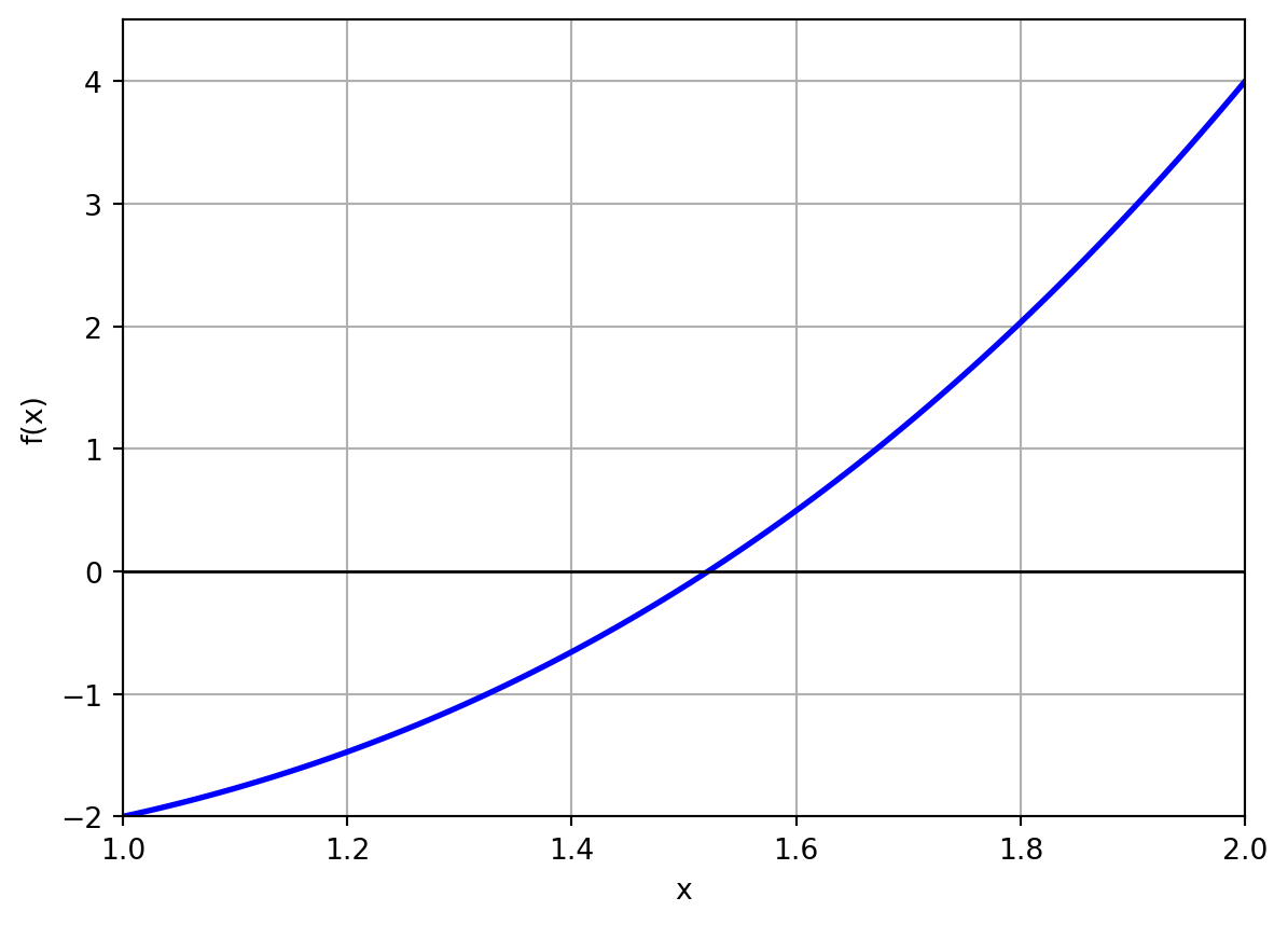
Consider the function $f(x) = x^3 - x - 2$. We want to find a root of this function in the interval $[1, 2]$. To help you, the graph of $f(x)$ on this interval is provided below.

Figure 3.8: Graph of $f(x) = x^3 - x - 2$.

Using the graph to roughly estimate function values, carry out the first three iterations of the Bisection Method. [3 marks]
The equation $x^3 - x - 2 = 0$ can be rewritten as a fixed-point problem $x = g(x)$ in several ways. Consider the rearrangement $g(x) = \sqrt[3]{x+2}$. We have $g(1) \approx 1.44$ and $g(2) \approx 1.58$.
1. Calculate the derivative $g'(x)$. Use it to show whether the fixed-point iteration $x_n = g(x_{n-1})$ is guaranteed to converge for any starting value $x_0 \in [1, 2]$. [3 marks]
2. Complete the following Python code to perform 10 iterations of the fixed-point iteration $x_n = g(x_{n-1})$ starting with $x_0 = 1.0$. [3 marks]

def fixed_point_iteration():
    x = 1.0
    for i in range(...):
        x = ...
    return x

Further reading: Section 2.2 of (Burden and Faires 2010).

Burden, Richard L., and J. Douglas Faires. 2010. Numerical Analysis. 9th ed. Brooks Cole.

You may find that we are going too slow for you and that you have the capacity and interest to learn more. In this case I can recommend the optional Appendix C on Numerical Linear Algebra.↩︎

Iteration	Width of Interval	Maximal Error
1	\(\|b-a\|\)	\(\frac{\|b-a\|}{2}\)
2	\(\frac{\|b-a\|}{2}\)
3	\(\frac{\|b-a\|}{2^2}\)
\(\vdots\)	\(\vdots\)	\(\vdots\)
\(n\)	\(\frac{\|b-a\|}{2^{n-1}}\)