Code
import matplotlib.pyplot as plt
import numpy as np
x = np.linspace(1, 4, 100)
plt.plot(x, np.log(x), label="log(x)")
plt.plot(x, np.sin(x), label="sin(x)")
plt.xlabel("x")
plt.legend()
plt.grid()
plt.show()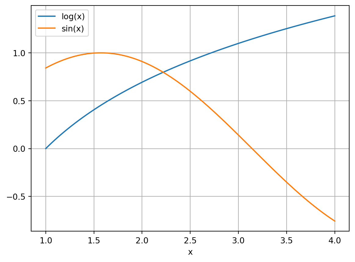
A Learning Guide
What I cannot create, I do not understand.
–Richard P. Feynman
Mathematics is not just an abstract pursuit; it is an essential tool that powers a vast array of applications. From weather forecasting to black hole simulations, from urban planning to medical research, from ecology to epidemiology, the application of mathematics has become indispensable. Central to this applied force is Numerical Analysis.
Numerical Analysis is the discipline that bridges continuous mathematical theories with their concrete implementation on digital computers. These computers, by design, work with discrete quantities, and translating continuous problems into this discrete realm is not always straightforward.
In this module, we will explore some key techniques, algorithms, and principles of Numerical Analysis that enable us to translate mathematical problems into computational solutions. We will delve into the challenges that arise in this translation, the strategies to overcome them, and the interaction of theory and practice.
Many mathematical problems cannot be solved analytically in closed form. In Numerical Analysis, we aim to find approximation algorithms for mathematical problems, i.e., schemes that allow us to compute the solution approximately. These algorithms use only elementary operations that computers know how to do (\(+,-,\times,/\)), but often a long sequence of them, so that in practice they need to be run on computers.
Solve the equation \[\log(x) = \sin(x)\] for \(x\) in the interval \(x \in (0,\pi)\). Stop and try using all of the algebra that you ever learned to find \(x\). You will quickly realize that there are no by-hand techniques that can solve this problem! A numerical approximation, however, is not so hard to come by. The following graph shows that there is a solution to this equation somewhere between \(x=2\) and \(x=2.5\).
import matplotlib.pyplot as plt
import numpy as np
x = np.linspace(1, 4, 100)
plt.plot(x, np.log(x), label="log(x)")
plt.plot(x, np.sin(x), label="sin(x)")
plt.xlabel("x")
plt.legend()
plt.grid()
plt.show()What if we want to evaluate
\[ \int_0^\pi \sin(x^2) dx? \]
import matplotlib.pyplot as plt
import numpy as np

def f(x):
    return np.sin(x**2)

a = 0
b = np.pi
n = 1000  # Number of points for numerical integration

x = np.linspace(a, b, n)
y = f(x)

# Calculate the numerical integral using the trapezoidal rule
integral = np.trapezoid(y, x)

# Shade the positive and negative regions differently
plt.fill_between(x, y, where=y>=0, color='green', alpha=0.5, label="Positive")
plt.fill_between(x, y, where=y<0, color='red', alpha=0.5, label="Negative")

# Plot the curve
plt.plot(x, y, color='black', label=r"$\sin(x^2)$")

# Set labels and title
plt.xlabel("x")

# Add legend
plt.legend()

# Show the plot
plt.grid()
plt.show()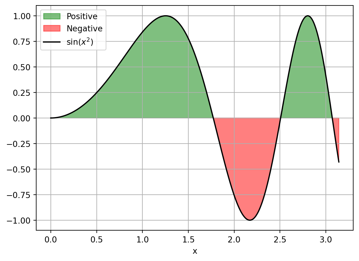
Again, trying to use any of the possible techniques for using the Fundamental Theorem of Calculus, and hence finding an antiderivative, on the function \(\sin(x^2)\) is completely hopeless. Substitution, integration by parts, and all of the other techniques that you know will all fail. Again, a numerical approximation is not so difficult and is very fast and gives the value
# Use Simpson's rule to approximate the integral of sin(x^2) from 0 to pi
from scipy.integrate import simpson
print(simpson(y, x = x))0.7726517138019184By the way, this integral (called the Fresnel Sine Integral) actually shows up naturally in the field of optics and electromagnetism, so it is not just some arbitrary integral that was cooked up just for fun.
Say we needed to solve the differential equation
\[\frac{dy}{dt} = \sin(y^2) + t.\]
The nonlinear nature of the problem precludes us from using most of the typical techniques (e.g. separation of variables, undetermined coefficients, Laplace Transforms, etc). However, computational methods that result in a plot of an approximate solution can be made very quickly. Here is a plot of the solution up to time \(t=2.5\) with initial condition \(y(0)=0.1\):
import matplotlib.pyplot as plt
import numpy as np
from scipy.integrate import solve_ivp

def f(t, y):
    return np.sin(y**2) + t

# Initial condition
y0 = 0.1

# Time span for the solution
t_span = (0, 2.5)

# Solve the differential equation using SciPy's solver
sol = solve_ivp(f, t_span, [y0], max_step=0.1, dense_output=True)

# Extract the time values and solution
t = sol.t
y = sol.sol(t)[0]

# Plot the numerical solution
plt.plot(t, y)

# Labels and title
plt.xlabel('t')
plt.ylabel('y')

# Show the plot
plt.grid(True)
plt.show()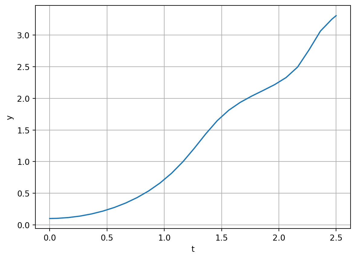
This was an artificial example, but differential equations are central to modelling the real world in order to predict the future. They are the closest thing we have to a crystal ball. Here is a plot of a numerical solution of the SIR model of the evolution of an epidemic over time:
import numpy as np
from scipy.integrate import odeint
import matplotlib.pyplot as plt

# SIR model differential equations
def sir_model(y, t, N, beta, gamma):
    S, I, R = y
    dSdt = -beta * S * I / N
    dIdt = beta * S * I / N - gamma * I
    dRdt = gamma * I
    return dSdt, dIdt, dRdt

# Total population, N
N = 1000
# Initial number of infected and recovered individuals
I0, R0 = 1, 0
# Everyone else is susceptible to infection initially
S0 = N - I0 - R0
# Contact rate, beta, and mean recovery rate, gamma, (in 1/days)
beta, gamma = 0.25, 1./20
# A grid of time points (in days)
t = np.linspace(0, 160, 160)

# Initial conditions vector
y0 = S0, I0, R0
# Integrate the SIR equations over the time grid, t
ret = odeint(sir_model, y0, t, args=(N, beta, gamma))
S, I, R = ret.T

# Plot the data on three separate curves for S(t), I(t) and R(t)
plt.figure(figsize=(10,6))
plt.plot(t, S, 'b', alpha=0.7, linewidth=2, label='Susceptible')
plt.plot(t, I, 'y', alpha=0.7, linewidth=2, label='Infected')
plt.plot(t, R, 'g', alpha=0.7, linewidth=2, label='Recovered')
plt.xlabel('Time /days')
plt.ylabel('Number (1000s)')
plt.ylim(0, N)
plt.title('SIR Model Simulation')
plt.legend()
plt.show()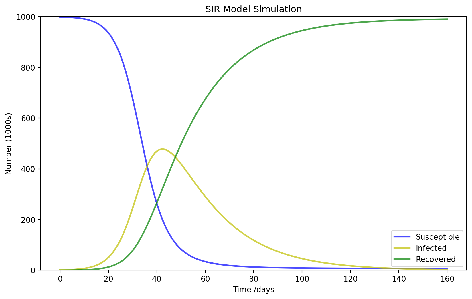
So why should you want to venture into Numerical Analysis rather than just use the computer as a black box?
Precision and Stability: Computers, despite their power, can introduce significant errors if mathematical problems are implemented without care. Numerical Analysis offers techniques to ensure we obtain results that are both accurate and stable.
Efficiency: Real-world applications often demand not just correctness, but efficiency. By grasping the methods of Numerical Analysis, we can design algorithms that are both accurate and resource-efficient.
Broad Applications: Whether your interest lies in physics, engineering, biology, finance, or many other scientific fields, Numerical Analysis provides the computational tools to tackle complex problems in these areas.
Basis for Modern Technologies: Core principles of Numerical Analysis are foundational in emerging fields such as artificial intelligence, quantum computing, and data science.
The prerequisites for this material include a firm understanding of calculus and linear algebra and a good understanding of the basics of differential equations.
By the end of this module, you will not merely understand the methods of Numerical Analysis; you will be equipped to apply them efficiently and effectively in diverse scenarios: you will be able to tackle problems in physics, engineering, biology, finance, and many other fields; you will be able to design algorithms that are both accurate and resource-efficient; you will be able to ensure that your computational solutions are both accurate and stable; you will be able to leverage the power of computers to solve complex problems.
There are 4 one-hour whole-class sessions every week. Three of these are listed on your timetable as “Lecture” and one as “Computer Practical”. However, in all these sessions you, the student, are the one that is doing the work; discovering methods, writing code, working problems, leading discussions, and pushing the pace. I, the lecturer, will act as a guide who only steps in to redirect conversations or to provide necessary insight. You will use the whole-class sessions to share and discuss your work with the other members of your group. There will also be some whole-class discussions moderated by me.
You will find that this text is not a set of lecture notes. Instead it mostly just contains collections of exercises with minimal interweaving exposition. It is expected that you do every one of the exercises in the main body of each chapter and use the sequencing of the exercises to guide your learning and understanding.
Therefore the whole-class sessions form only a very small part of your work on this module. For each hour of whole-class work you should timetable yourself about two and a half hours of work outside class for working through the exercises on your own. I strongly recommend that you put those two and a half hours (ten hours spread throughout the week) into your timetable.
In order to enable you to get immediate feedback on your work also in between class sessions, I have made feedback quizzes where you can test your understanding of the material and your results from some of the exercises. Exercises that have an associated question in the feedback quiz are marked with a 🎓.
There are no traditional problem sheets in this module. In this module you will be working on exercises continuously throughout the week rather than working through a problem sheet only every other week.
At the end of each chapter there is a section entitled “Problems” that contains additional exercises aimed at consolidating your new understanding and skills. These are optional. Many of the chapters also have a section entitled “Projects”. These projects are more open-ended investigations, designed to encourage creative mathematics, to push your coding skills and to require you to write and communicate mathematics. These projects are entirely optional and perhaps you will like to return to one of these even after the module has finished. If you do work on one of the projects, be sure to share your work with me at gustav.delius@york.ac.uk because will be very interested, also after the end of the module.
If you notice any mistakes or unclear things in the learning guide, please point them out to me in the class sessions or at gustav.delius@york.ac.uk. Many thanks go to Ben Mason and Toby Cheshire for the corrections they had sent in for a previous version of this guide.
You will need two notebooks for working through the exercises in this guide: one in paper form and one electronic. Some of the exercises are pen-and-paper exercises (and often these are marked with a pen icon ✏️) while others are coding exercises (often marked with a computer icon 💻) and some require both writing or sketching and coding. You can keep your two notebooks linked through the numbering of the exercises. There are also some exercises that are marked with a Discussion icon 💬. These are exercises that you should be discussing with other members of your group.
You will keep your coding notebooks in Google Colab, which we will discuss below. Most students find it easiest to have one dedicated Colab notebook per section, but some students will want to have one per chapter. You are highly encouraged to write explanatory text into your Google Colab notebooks as you go so that future-you can tell what it is that you were doing, which problem(s) you were solving, and what your thought processes were.
In the end, your collection of notebooks will contain solutions to every exercise in the guide and can serve as a reference manual for future numerical analysis problems. At the end of each of your notebooks you may also want to add a summary of what you have learned, which will both consolidate your learning and make it easier for you to remind yourself of your new skills later.
One request: do not share your notebooks publicly on the internet because that would create temptation for future students to not put in the work themselves, thereby robbing them of the learning experience.
If you have a computer, bring it along to the class sessions. However this is not a requirement. I will bring along some spare machines to make sure that every group has at least one computer to use during every session. The only requirements for a computer to be useful for this module is that it can connect to the campus WiFi, can run a web browser, and has a physical keyboard (typing code on virtual keyboards is too slow). The “Computer Practical” takes place in a PC classroom, so there will of course be plenty of machines available then.
Unfortunately, your learning in the module also needs to be assessed. The final mark will be made up of 40% coursework and 60% final exam.
The 40% coursework mark will come from 10 short quizzes that will take place during the “Computer practical” in weeks 2 to 11. Answering each quiz should take less than 5 minutes but you will be given 16 minutes each to complete the quizzes in order to give you a large safety margin and remove stress. Late answers will not be accepted. The quizzes will be based on exercises that you will already have worked through and for which you will have had time to discuss them in class, so they will be really easy if you have engaged with the exercises as intended. Each quiz will be worth 5 points. There will be a practice quiz in the computer practical in week 1.
While working on the assessment quizzes you can already check your answers. If one of your answers is incorrect you can correct it and submit it again. However this will attract a penalty of 30% of the total mark for that answer. For multiple choice questions the penalty for a wrong answer may be even higher to discourage guessing. So it pays to be careful.
During the assessment quizzes you will be required to work exclusively on one of the PCs in the computer practical room rather than your own machine. This means in particular that you need to be physically present for the assessment. While working on the quiz you are only allowed to use a web browser, and the only pages you are allowed to have open are this guide, the quiz page on Moodle and any of your notebooks on Google Colab, with the AI features switched off. You are not allowed to use any AI assistants or other web pages. Besides your digital notebooks on Google Colab you may also use any hand-written notes as long as you have written them yourself.
To allow for the fact that there may be weeks in which you are ill or otherwise prevented from performing to your best in the assessment quizzes, your final coursework mark will be calculated as the average over your 8 best marks. If exceptional circumstances affect more than two of the 10 quizzes then you would need to submit an exceptional circumstances claim.
The 60% final exam will be a 2 hour exam of the usual closed-book form in an exam room during the exam period. To prepare yourself for the final exam, there will be an exam style question at the end of each chapter, and I will make a practice exam available at the end of the module.
In this module we will only scratch the surface of the vast subject that is Numerical Analysis. The aim is for you at the end of this module to be familiar with some key ideas and to have the confidence to engage with new methods when they become relevant to you.
There are many textbooks on Numerical Analysis. Standard textbooks are (Burden and Faires 2010) and (Kincaid and Cheney 2009). They contain much of the material from this module. A less structured and more opinionated account can be found in (Acton 1990). Another well known reference that researchers often turn to for solutions to specific tasks is (Press et al. 2007). You will find many others in the library. They may go also under alternative names like “Numerical Methods” or “Scientific Computing”.
You may also want to look at textbooks for specific topics covered in this module, like for example (Butcher 2016) for methods for ordinary differential equations.
You have the following jobs as a student in this module:
Fight! You will have to fight hard to work through this material. The fight is exactly what we are after since it is ultimately what leads to innovative thinking.
Screw Up! More accurately, do not be afraid to screw up. You should write code, work problems, and develop methods, then be completely unafraid to scrap what you have done and redo it from scratch.
Collaborate! You should collaborate with your peers, both within your group and across the whole class. Discuss exercises, ask questions, help others.
Enjoy! Part of the fun of inquiry-based learning is that you get to experience what it is like to think like a true mathematician / scientist. It takes hard work but ultimately this should be fun!
To properly understand numerical analysis, you will need to write code in order to experiment with the methods we discuss. You will be using Python for this purpose. or most of you, coding in Python will not be new. For example, you have probably seen it in your first year “Mathematical Programming & Skills” module. But perhaps you have never seen Python before. You will have some notion of what a programming language “is” and “does”, but you may never have written any code. That is all right. You will pick it up as you go along.
Appendix A — Python covers some of the basics of Python programming that we will use in this module. If you are new to Python, don’t feel that you need to work through this appendix in one go. Instead, spread the work over the first two weeks of the course and interlace it with your work on the first two chapters.
Every computer is its own unique flower with its own unique requirements. Hence, we will not spend time here giving you all of the ways that you can install Python and all of the associated packages necessary for this module. Instead I ask that you use the Google Colab notebook tool for writing and running your Python code: https://colab.research.google.com.
Google Colab allows you to keep all of your Python code on your Google Drive. The Colab environment is a free and collaborative version of the popular Jupyter notebook project. Jupyter notebooks allow you to write and test code as well as to mix writing (including LaTeX formatting) in along with your code and your output. I recommend that if you are new to Google Colab, you start by watching the brief introductory video.
Now the time has come for the first two exercises of this module.
Exercise 1 💻 Spend a bit of time poking around in Colab. Figure out how to
Create new Colab notebooks.
Add and delete code cells.
Type a simple calculation like 1+1 into a code cell and evaluate it.
Add and delete text cells.
Add an equation to a text cell using LaTeX notation.
Save a notebook to your Google Drive.
Open a notebook from Google Drive.
Share a notebook with other members of your group and see if you can collaboratively edit it.
Exercise 2 💻 Click on this link to a Colab notebook. It should open it in Colab. Then save a copy of it to your Google Drive. You need a copy because you will not have permission to edit the original. Follow the instructions in the notebook.
You will have gathered from the previous exercise that in this module you are not only allowed to use AI, you are encouraged to use AI. However you have probably already discovered that you get more out of an AI if you are already familiar with the basic concepts of a subject. You will need to be able to understand and check any answer an AI gives you. If there is something in an AI answer that is not totally clear or not obviously correct, always ask the AI to explain the details of its answer and ask follow-on questions until everything is crystal-clear.
During the 10 assessment quizzes you will not be allowed to use any AI. In particular you will be required to switch off the AI features in Google Colab. It is thus a good idea when working on practice exercises to also switch off the AI features to make sure you know what you are doing even when there is no AI assistance. To switch off the AI features you should tick the “Hide generative AI” checkbox on the “AI assistance” tab of the “Settings” page in Google Colab. 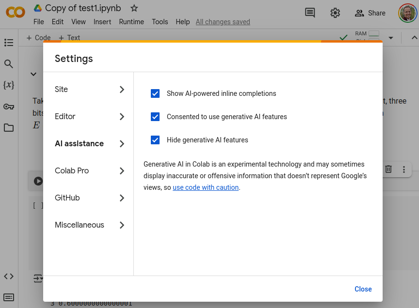
Exercise 3 💻 I am interested to learn more about you to help me make this module work well for you. It would be helpful if you would answer the questionnaire at https://forms.gle/YHHExaAnVzcLtBcU7. Of course you are free to share as much or as little as you like.
© Gustav Delius. This learning guide is licensed under a Creative Commons Attribution-NonCommercial-ShareAlike 4.0 International License. You may copy, distribute, display, remix, rework, and perform this copyrighted work, as long as you give credit to Gustav Delius gustav.delius@york.ac.uk and to the late Eric Sullivan, formerly Mathematics Faculty at Carroll College, on whose learning guide this one is based.