2 Discrete-time population models
So far we have assumed that the rate of change of the population number has no explicit time dependence. However births and also deaths often happen on an annual cycle. Many fish have their spawning season in the spring, and many birds breed in the summer and annual plants produce their seed and then die in winter. In this case, the rate of change of the population number is not constant, but depends on the time of the year. We can model this by introducing a time dependence in the birth and death rates. However this will lead to equations that will be difficult to analyse. Instead we can give up on the idea of modelling the population numbers continuously through time and instead only follow how the population changes from year to year.
So we will use models of the form \[ N_{t+1} = f(N_t) \tag{2.1}\] where \(N_t\) is the population number at time \(t\) and \(f\) is some function. Time \(t\) now takes on only integer values, and the population number is only defined at these times. This is called a discrete-time model. Given the initial population number \(N_0\), we can calculate the population number at any future time \(t\) by iterating the function \(f\): \(N_1 = f(N_0)\), \(N_2 = f(N_1)=f(f(N_0)),\ldots N_t = f(f(\ldots f(N_0)\ldots))\).
Learning Objectives
After completing this chapter, you should be able to:
- Mathematical Modeling
- Write down difference equations for population dynamics
- Identify and interpret key parameters in discrete-time models
- Solve basic discrete-time population models
- Model Analysis
- Find fixed points of discrete-time models
- Determine stability using linear analysis and cobweb diagrams
- Interpret cobweb diagrams
- Predict long-term behavior of populations
- Bifurcations
- Identify different types of bifurcations in discrete-time models
- Analyze how model behavior changes at bifurcation points
- Understand period-doubling bifurcations unique to discrete systems
- Applications
- Compare and contrast different discrete-time population models
- Analyze harvesting strategies in discrete-time models
- Understand critical depensation in discrete systems
Key Ecological Concepts
Before diving into the mathematical models, let’s clarify some ecological terminology:
- Population: A group of individuals of the same species living in a particular area
- Carrying capacity: The maximum sustainable population size in a given environment
- Critical depensation: A threshold effect where populations below a certain size tend to decline to extinction
- Density dependence: How population growth rates change with population size
- Seasonal reproduction: When breeding occurs at specific times of year rather than continuously
These concepts will help explain why we choose particular mathematical forms for our models.
2.1 Exponential model
Just as we started with the exponential model in Chapter 1, we begin here with the simplest discrete-time model \[ N_{t+1} = R N_t \tag{2.2}\] where \(R>0\) is the growth factor. This is the discrete-time version of the continuous-time exponential model. The solution to this equation is \[ N_t = N_0 R^t. \tag{2.3}\] It is important to stress that \(R\) is not a growth rate but a dimensionless growth factor. Comparing the discrete-time solution to the continuous-time solution \(N(t)=N_0\exp(rt)\) we see that they agree at integer times \(t\) if we measure time in years and set \[ R=\exp(r \cdot 1\text{ year}). \tag{2.4}\] If you are confused by the units, remember that the exponential function is dimensionless, so the argument of the exponential function must be dimensionless. We need the extra factor of 1 year because \(r\) is a rate and has dimension 1/time.
The population number grows exponentially with time if \(R>1\) and declines exponentially if \(R<1\). To get more realistic models we again need to introduce a limited carrying capacity.
Exercise 2.1 (AER) You may be familiar with the distinction between the instantaneous rate \(r\) in a continuous-time model and the annual equivalent rate \(R\) in the corresponding discrete-time model from your savings account. Assuming that the bank pays interest into your account but you do not withdraw any money, what interest rate \(r\) do you need so that the money has increased by 5% after one year, i.e., so that the yearly growth factor is \(R=1.05\)?
2.2 Logistic model
Recall how we introduced the continuous-time logistic model by assuming that the per-capita birth rate declines linearly with the population number and vanishes when the population reaches its carrying capacity. This gave us the equation \[ \frac{dN}{dt} = rN\left(1 - \frac{N}{K}\right) \tag{2.5}\] where \(r\) is the per-capita growth rate and \(K\) is the carrying capacity.
It turns out that there are several models which all deserve to be called the discrete-time logistic model. The most famous discrete-time logistic model is the Verhulst model:
\[ \begin{split} N_{t+1} &=N_t + R_0 N_t\left(1 - \frac{N_t}{K}\right)\\ &= (R_0+1)N_t\left(1 - \frac{N_t}{K(R_0+1)/R_0}\right)\\ &= RN_t\left(1-\frac{N_t}{\tilde{K}}\right)=f(N_t), \end{split} \tag{2.6}\] We have written the model in two alternative forms, with \(R=R_0+1\) and \(\tilde{K}=K(R_0+1)/R_0\), because the first form makes it easier to read off the fixed point, while the second form makes the analogy with the continuous-time logistic model more obvious. Eq. 2.6 is also often referred to as the logistic map and is a famous example of a chaotic system.
Again it is important to stress that \(R_0\) is not a growth rate but a dimensionless growth factor. We are interested in the case where \(R_0>0\) and \(K>0\).
A fixed point is a value for which \(N_{t+1}=N_t\), i.e. a value of \(N\) for which the population number does not change from year to year. Thus it is a value \(N^*\) for which \(f(N^*)=N^*\). Using the second form of the model, we can see easily that the fixed points are \(N^*=0\) and \(N^*=K\), so \(K\) is the carrying capacity.
2.3 Linear stability analysis
We now want to study the stability of the fixed points in discrete-time models. As discussed, fixed points \(N^*\) satisfy the equation \(N^*=f(N^*)\). We study the stability of the fixed points by looking at the sequence \(N_t\) for \(t\) close to the fixed point. That means we write \(N(t)=N^*+n_t\) for \(n_t<<1\). We then have \[ \begin{split} N_{t+1} = N^*+n_{t+1}=f(N_t) = f(N^*+n_t) = f(N^*) + f'(N^*)n_t + \ldots \end{split} \tag{2.7}\] where we have used the Taylor expansion of \(f\) around \(N^*\). Because \(N^*\) is a fixed point, we have \(f(N^*)=N^*\). Thus we find that \[ n_{t+1} \approx f'(N^*)n_t \tag{2.8}\] where we neglected the higher order terms in the Taylor expansion. This is a linear equation for \(n_t\) that we know how to solve: \[ n_t = n_0 (f'(N^*))^t. \tag{2.9}\] So we have found that:
If \(|f'(N^*)|<1\), then \(n_t\) will decrease with time and the fixed point is stable.
If \(|f'(N^*)|>1\), then \(n_t\) will increase with time and the fixed point is unstable.
If \(|f'(N^*)|=1\), then we cannot say anything about the stability of the fixed point from this analysis.
Exercise 2.2 (+ Stability in Verhulst model) Use the stability criterion that we just derived to derive a condition on the parameter \(R_0\) of the Verhulst model that makes the non-zero fixed point \(N^*=K\) a stable fixed point.
2.4 Cobweb diagrams
In the continuous-time case we also had a graphical way to see the stability of fixed points. We will now introduce a graphical method for studying the stability of fixed points in discrete-time models, called the cobweb method.
We plot the function \(f(N_t)\) and the line \(N_{t+1}=N_t\). The fixed points are the intersection points of the function and the line. We then draw the graph of the sequence \(N_t\) by starting at the initial population number \(N_0\) and iterating the function \(f(N_t)\) to find \(N_1\), then iterating the function again to find \(N_2\), and so on. The graph of the sequence \(N_t\) is called the cobweb. The stability of the fixed points can be read off from the cobweb. If the cobweb spirals into the fixed point, as shown in Figure 2.1, then the fixed point is stable. If the cobweb spirals out of the fixed point, as shown in Figure 2.2, then the fixed point is unstable. You have to press the play button below the figures to see the cobweb diagrams in action.
The oscillatory nature of the sequence \(N_t\), hopping from one side of the fixed point to the other, that creates the cobweb pattern is due to the fact that the slope of \(f\) is negative at the fixed point. Ecologically, what is happening as the growth factor increases through \(R=3\) is that in a single year the population grows so much that it exceeds its carrying capacity. That then leads to unfavourable conditions in the following year, leading to a decrease below carrying capacity. Such oscillations in population numbers are not possible in a continuous-time model for a single un-structured population.
In Figure 2.1 the oscillations get damped over time and the system evolves towards a steady state. In Figure 2.1 the system evolves towards a state where the population number oscillates between two values. This is called a period-two orbit. We will have more to say about this in Section 2.7.
The graphical method for visualising the iterations will work also when the slope is positive at the fixed point, but it will not look like a cobweb because the system will not be oscillating around the fixed point but will be evolving towards it. Figure 2.3 shows the cobweb for a stable fixed point with positive slope \(0<f'(N^*)<1\) and Figure 2.4 shows the cobweb for an unstable fixed point with positive slope \(f'(N^*)>1\).
Exercise 2.3 (+ Verhulst model) For some choices of the parameters, the Verhulst model \[ N_{t+1}=RN_t\left(1-\frac{N_t}{\tilde{K}}\right) \tag{2.10}\] can lead to negative population numbers even when initially starting with a positive population below its carrying capacity. Derive the condition on the parameters for this to happen. One good way to approach this is to think about what the cobweb diagram would have to look like for such a scenario.
2.5 Other models with limited carrying capacity
You showed in Exercise 2.3 that the Verhulst model has the disadvantage that it can give negative population numbers. There are several other models that are discrete-time versions of the logistic model and do not have this problem. We will now look at the two most important of them.
2.5.1 Ricker model
Many fish species, like salmon, have distinct breeding seasons and their reproduction shows strong density dependence - when population density is too high, fewer offspring survive due to competition for spawning sites. The Ricker model captures this behavior through the equation:
\[ N_{t+1} = N_t\, e^{R_0\left(1 - \frac{N_t}{K}\right)}. \tag{2.11}\]
By moving the logistic factor inside the exponential, the Ricker model prevents negative population numbers. The fixed points are still \(N^*=0\) and \(N^*=K\). Ricker introduced this model to describe salmon populations.
Exercise 2.4 (* Ricker model) Find the fixed points in the Ricker model \[ N_{t+1} = N_t\, e^{R_0\left(1 - \frac{N_t}{K}\right)}. \tag{2.12}\] and investigate their stability. Do this both analytically and by drawing cobweb diagrams. Allow also negative values of \(R_0\) in your analysis, even though this is not ecologically realistic. Note that you will then need at least three cobweb diagrams because there are then two bifurcations.
2.5.2 Beverton-Holt model
The Beverton-Holt model, introduced by Ray Beverton and Sidney Holt in 1957, was developed to understand fish population dynamics. The model arose from their groundbreaking work on sustainable fisheries management while working at the Fisheries Laboratory in Lowestoft, UK. They were particularly interested in how the number of young fish (recruits) entering a population depends on the number of parent fish (spawning stock).
They proposed the model
\[ N_{t+1} = \frac{R N_t}{1 + \frac{R-1}{K}N_t}. \tag{2.13}\]
This has been a very influential model in fisheries science. On the face of it the model does not look very similar to the logistic model, but we will see the relationship when we solve the model. The trick is to make a change of variables from \(N_t\) to \(u_t = 1/N_t\). Then we have \[ u_{t+1} = \frac{1}{N_{t+1}} = \frac{1 + \frac{R-1}{K}N_t}{R N_t} = \frac{u_t}{R} + \frac{R-1}{R K}. \tag{2.14}\] This is a linear equation for \(u_t\), and linear equations are easy to solve. The easiest way to proceed is to look at the first few terms of the sequence \(u_t\) and guess the general form of the solution. We find \[\begin{split} u_1 &= \frac{u_0}{R} + \frac{R-1}{R K},\\ u_2 &= \frac{u_0}{R^2} + \frac{R-1}{R K}\left(1 + \frac{1}{R}\right),\\ u_3 &= \frac{u_0}{R^3} + \frac{R-1}{R K}\left(1 + \frac{1}{R} + \frac{1}{R^2}\right),\\ &\vdots\\ u_t &= \frac{u_0}{R^t} + \frac{R-1}{R K}\left(1 + \frac{1}{R} + \frac{1}{R^2} + \ldots + \frac{1}{R^{t-1}}\right). \end{split} \tag{2.15}\] The sum in the second term is a geometric series. We know the general formula for a geometric series: \[ 1 + x + x^2 + \ldots + x^{t-1} = \frac{1 - x^t}{1 - x}. \tag{2.16}\]
We can use this with \(x=1/R\) to sum terms in the second term. We find \[ u_t = \frac{u_0}{R^t} + \frac{R-1}{R K}\frac{1 - (1/R)^t}{1 - 1/R}. \] We simplify this a bit and bring everything on the same denominator. \[ u_t = \frac{u_0}{R^t} - \frac{(1/R)^t-1}{K} =\frac{Ku_0-1+R^t}{KR^t}. \tag{2.17}\]
We can now change back to \(N_t=1/u_t\) to find the solution to the Beverton-Holt model. We find \[ \begin{split} N_t &= \frac{1}{u_t}=\frac{K R^t}{Ku_0-1+R^t}\\ &=\frac{K/u_0}{KR^{-t}-R^{-t}/u_0+1/u_0}\\ &=\frac{KN_0}{N_0+(K-N_0)R^{-t}}. \end{split} \tag{2.18}\]
This is the solution to the Beverton-Holt model. Comparing this to the solution of the continuous-time logistic model from Eq. 1.5, \[ N(t) = \frac{KN_0}{N_0+(K-N_0)\exp(-rt)}, \tag{2.19}\] we see that they agree at integer times \(t\) if we measure time in years and set \(R=\exp(r \cdot 1\text{ year}).\)
Exercise 2.5 (Beverton-Holt model) Find the fixed points in the Beverton-Holt model \[ N_{t+1} = \frac{R N_t}{1 + \frac{R-1}{K}N_t}. \tag{2.20}\] and investigate their stability. Do this both analytically and by drawing cobweb diagrams.
2.6 Discrete-time harvesting model
We will now look at an example of a discrete-time model with harvesting and apply the techniques we have learned. The model has the standard discrete-time model form \(N_{t+1}=f(N_t)\), where \(f\) in our example is \[ f(N) = \frac{b N^2}{1+N^2}-EN. \tag{2.21}\] The constant \(b>2\) determines the growth rate of the population and the harvesting rate is determined by the harvesting effort \(E\).
We start by studying the model without harvesting, so we set \(E=0\) for now. As usual, we start by looking at the steady states of the model. The fixed points are the solutions to the equation \[ N^* = \frac{b\,{N^*}^2}{1+{N^*}^2}. \tag{2.22}\] There is the obvious solution \(N^*=0\). We can then find the non-zero solutions by dividing both sides by \(N^*\) and multiply them by \(1+{N^*}^2\) to get the equation \[ 1+{N^*}^2 = bN^*. \tag{2.23}\] This is a quadratic equation for \(N^*\), which we could rewrite in the more conventional form \[ {N^*}^2 - bN^* + 1 = 0. \tag{2.24}\] The solutions to this equation are \[ N^*_\pm = \frac{b\pm\sqrt{b^2-4}}{2}. \tag{2.25}\] The solutions are real if \(b^2-4\geq 0\), i.e. if \(b\geq 2\), which we have stipulated earlier. Both solutions are positive.
We now have enough information to draw a good sketch to understand the dynamics of the model. We can draw the function \(f(N)\) and the line \(N_{t+1}=N_t\). It may not be immediately obvious what the sketch of \(f(N)=bN^2/(1+N^2)\) looks like. We’ll reason ourselves through this in steps:
First let us consider what happens near \(N=0\). There the function is approximately \(f(N)\approx bN^2\). This is a parabola that opens upwards. The function is zero at \(N=0\) and increases quadratically with \(N\).
Next we consider what happens as \(N\) becomes large. There the function is approximately \(f(N)\approx b\). So the graph has a horizontal asymptote at \(y=b\).
We know that in between there are two fixed points. That means the graph needs to cross the diagonal line \(y=N\) twice.
Finally we observe that the function is monotonically increasing.
If we now draw something that has all these features, we will have a sufficiently good sketch of the function for our purpose of understanding the dynamics of the model. We will necessarily end up with something that qualitatively looks like the graph in Figure 2.5.
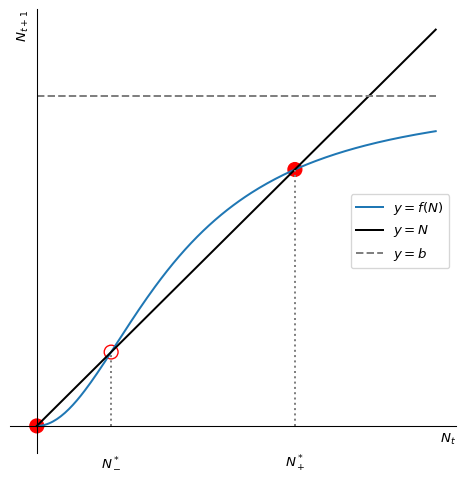
Using our cobweb technique, or simply looking at the slope of \(f\) at the fixed points, we can easily convince ourselves that the extinction fixed point is stable, the smaller non-zero fixed point \(N^*_-\) is unstable and the larger fixed point \(N^*_+\) is stable. in Figure 2.5 we have indicated the stable fixed points by solid circles and the unstable fixed points by open circles. So when the population number is larger than \(N^*_-\) it will grow towards \(N^*_+\), and when it is smaller than \(N^*_-\) it will go extinct. So this model exhibits a strong Allee effect with critical depensation. \(N^*_-\) is the smallest viable population size.
We can now add harvesting to the model. The extra term in the function \(f(N)\) is \(-EN\). This lowers the graph of \(f(N)\) by an amount that grows linearly with \(N\). This is illustrated in Figure 2.6.
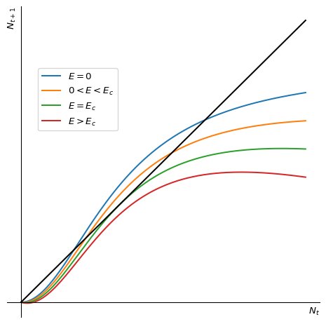
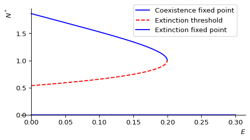
We see that as the harvesting effort \(E\) increases, the two fixed points move closer together. At a critical value \(E_c\) the two fixed points merge and disappear. The population number will then go extinct for all initial population numbers.
Let us find the critical value \(E_c\). For that we first determine the location of the fixed points in the presence of harvesting. So we solve the equation \[ N^* = \frac{b\,{N^*}^2}{1+{N^*}^2}-EN^*. \tag{2.26}\] Again this has a solution \(N^*=0\). We can then find the non-zero solutions by dividing both sides by \(N^*\) and multiply them by \(1+{N^*}^2\) to get the equation \[ (1+E){N^*}^2-bN^*+1+E = 0. \tag{2.27}\] This is solved by \[ N^*_\pm = \frac{\frac{b}{1+E}\pm\sqrt{\left(\frac{b}{1+E}\right)^2-4}}{2}. \tag{2.28}\]
We see that these solutions are real only if \(\left(\frac{b}{1+E}\right)^2-4\geq 0\), i.e., if \(E< \frac{b-2}{2}\). Thus the critical effort is \(E_c=\frac{b-2}{2}\). Fishing above this level will lead to extinction of the population. But even fishing just near this level is risky because the population number will be very close to the minimum viable population and a small disturbance could lead to extinction.
2.7 Period-doubling route to chaos
Take another look at Figure 2.1 and Figure 2.2. Just a little change in the function \(f(N)\) changed the nature of the fixed point. Such a change can be the consequence of a small change in a model parameter, for example the intrinsic growth rate.
We will use the logistic map to illustrate the period-doubling route to chaos, although the phenomenon is more general. The logistic map is a simple discrete-time model for population growth that exhibits a period-doubling route to chaos. It is defined as \[ X_{t+1} = R\,X_t\,(1-X_t) =: f(X_t). \tag{2.29}\] It is the same as the Verhulst model Eq. 2.6, just written in terms of \(X_t = N_t/\tilde{K}\). Figure 2.8 shows the graph of \(f(X)\) of the Verhulst model at three different values of the intrinsic growth factor \(R\). For \(R=2.8\) the slope of \(f\) at the fixed point is less steep than \(-1\) and thus the fixed point is stable, as in Figure 2.1. For \(R=3.2\) the slope of \(f\) at the fixed point is steeper than \(-1\) and thus the fixed point is unstable and the population number starts to oscillate, as in Figure 2.2. At \(R=3\) the system switches from one behaviour to the other. That is the bifurcation point.
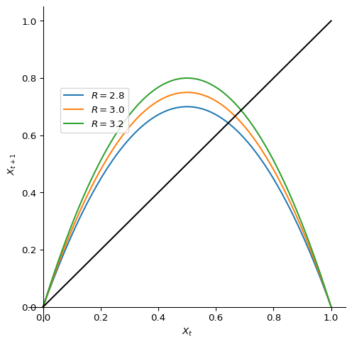
Figure 2.9 shows a simplified bifurcation diagram for the Verhulst model. A bifurcation diagram shows the location of fixed points or periodic orbits, with stable fixed points or stable periodic orbits represented by solid lines and unstable fixed points or unstable periodic orbits represented by dashed lines. Reading the diagram from left to right, which corresponds to increasing growth factor \(R\) in the Verhulst model, we see how at first the stable fixed point (which is located at the carrying capacity \(K\)) moves towards larger population sizes. At \(R=3\) it becomes unstable and spawns a stable periodic orbit whose amplitude grows until that periodic orbit itself becomes unstable, in another period-doubling bifurcation.
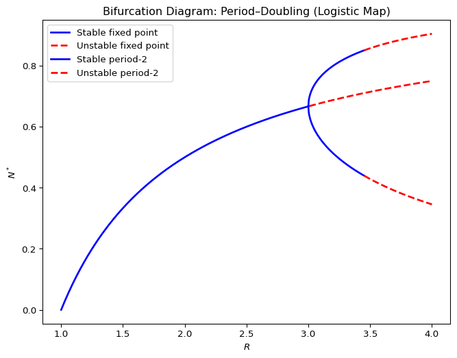
Figure 2.9 does not show the period 4 orbit that emerges when the period 2 orbit becomes unstable. The full diagram quickly becomes very messy as \(R\) increases, as shown in Figure 2.10. Period-doubling cascades continue until the system enters a chaotic regime for \(R>3.56995\).
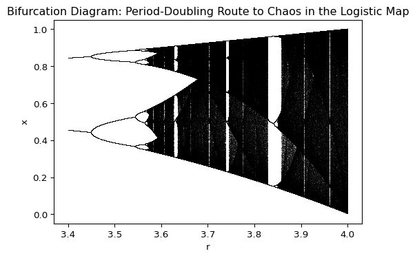
In the chaotic regime the system displays highly sensitive dependence on initial conditions, where small differences in the starting population can result in vastly different outcomes over time. The period-doubling route to chaos, as seen in the logistic map, is a classic example of how simple nonlinear equations can produce complex and unpredictable behavior. How important chaos is for ecological systems is a subject of ongoing debate.
2.8 Bifurcations
As mentioned before, a bifurcation is a change in the existence and stability of fixed points or periodic orbits as the parameters of the model are varied. You have met bifurcations in continuous-time models already in your Classical Dynamics module. You have seen there that in one-dimensional systems described by a single ODE there are three different types of bifurcation: saddle-node, pitchfork, transcritical. The same types of bifurcations can occur in discrete-time models and we will discuss and visualise each of these bifurcation types below. These bifurcations happen if there is a fixed point with \(f'(N^*)=1\). Then there is also one more type: the period-doubling bifurcation, which happens when \(f'(N^*)=-1\), and which we have met in Section 2.7.
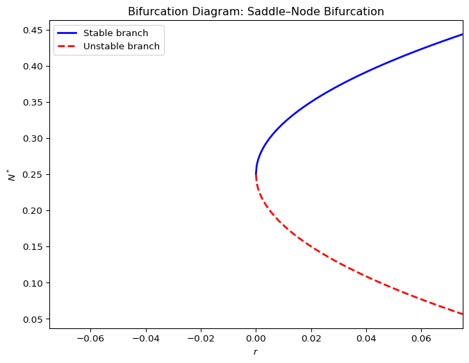
2.8.1 Saddle-node bifurcation
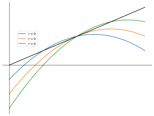
We have already seen a saddle-node bifurcation in the discrete-time harvesting mode, where two fixed points merge and disappear as the parameter is varied. This is also sometimes referred to as a tangent bifurcation. Figure 2.11 shows an example of a function \(f(N)\) that depends on a parameter \(r\) in such a way that for \(r>0\) the graph of \(f(N)\) crosses the diagonal twice, which means that there are two fixed points. Then at exactly \(r=0\) the function is tangent to the diagonal, i.e, there is only a single fixed point. Then for \(r<0\) the function does not touch the diagonal so that there are no fixed points left.
<Figure size 768x576 with 0 Axes>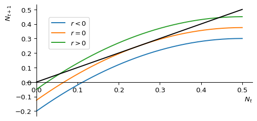
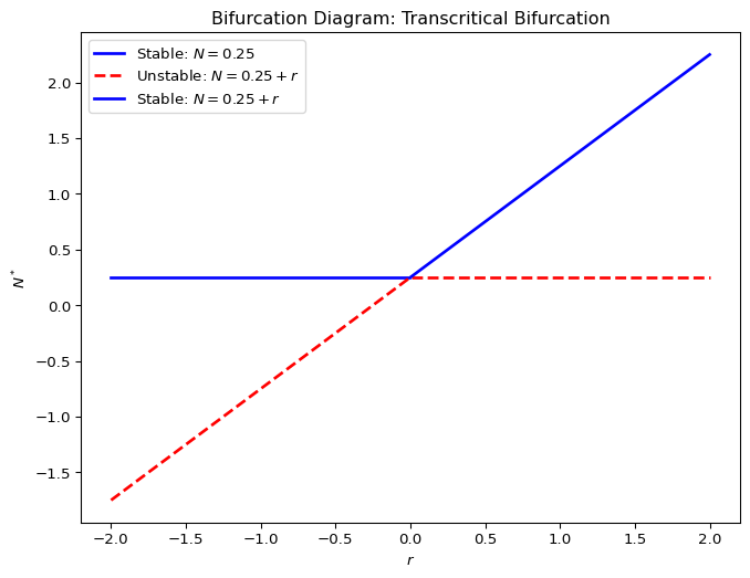
Figure 2.12 shows the corresponding bifurcation diagram.
2.8.2 Transcritical bifurcation
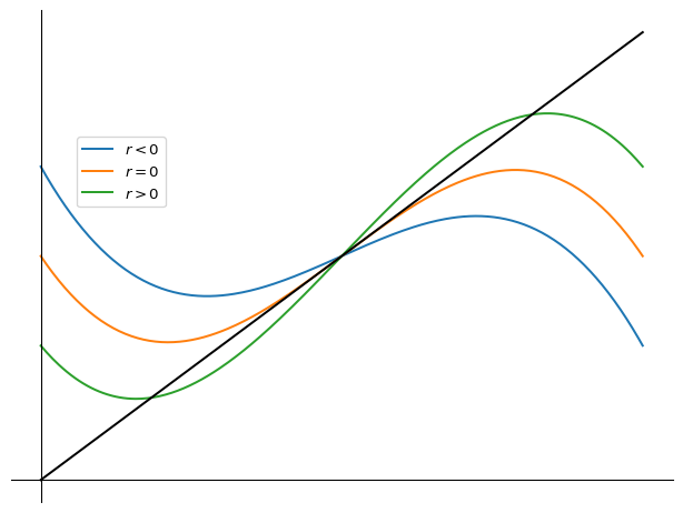
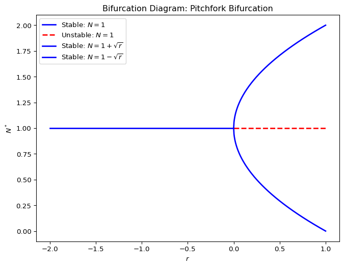
2.8.3 Pitchfork bifurcation
Exercise 2.6 (o House finches) [Note: in this problem we combine a continuous time model for the dynamics within a single year with a discrete model for the dynamics from one year to the next. The subscript \(t \in \mathbb{Z}\) refers to the discrete year whereas \(\tau\in\mathbb{R}\) will indicate the continuous time within a single year.]
A population of house finches resides in an isolated region in North America. In this problem you want to find out about the long-term prospects for the population.
Each year the males and females begin their search for mates at the beginning of winter with a combined population number \(N_t\) in year \(t\), and form \(P_t\) breeding pairs by the end of this search period, the start of the breeding season.
The mate search period lasts from within-year time \(\tau = 0\) to the end of the search period at within-year time \(\tau = T\). Assume that there is a 1:1 sex ratio and that males \(M(\tau)\) and females \(F(\tau)\) locate one another randomly to make a pair at rate \(\sigma\), such that the number \(M(\tau)\) of males that are not in a pair at time \(\tau\) satisfies \[\frac{dM}{d\tau}=-\sigma \,M\,F \] and similarly the number \(F\) of females that are not in a pair at time \(\tau\) satisfies \[\frac{dF}{d\tau}=-\sigma \,M\,F. \]
You are given that the number of breeding pairs that establish a nest and breed successfully is \(G(P_t)P_t\), where the fraction \(G(P_t)\) takes the particular form \[G(P_t) = \frac{1}{1+P_t/\delta},\] where \(\delta\) represents the density of available nesting sites. Each pair that reproduces successfully has a mean number \(c\) of offspring.
The probability that a bird will survive from one year to the next is \(s\).
Show that the number \(n(\tau)=M(\tau)+F(\tau)\) of birds not in a pair is governed by \[\frac{dn}{d\tau}=-\frac{\sigma}{2}n^2, ~~~n(0)=N_t.\]
Using the above, show that the number \(n(T)\) of birds that have not found a mate at the start of the breeding season in year \(t\) is \[n(T)=\frac{r\,N_t}{r+2N_t}\] where \(N_t\) is the number of birds at the start of the season in that particular year and where \(r=4/(\sigma T)\).
Explain why the number of pairs \(P(\tau)\) is governed by \[\frac{dP}{d\tau}=-\frac12\frac{dn}{d\tau},~~~P(0)=0.\]
Use the above to show that the number of breeding pairs at the start of the breeding season in year \(t\) is \[P_t:=P(T)=\frac{N_t^2}{r+2N_t}.\]
Show that the population \(N_{t+1}\) at the beginning of winter in year \(t+1\) is given by \[ N_{t+1}=s\,N_t+\frac{c\,N_t^2}{r+2N_t+N_t^2/\delta}. \tag{2.30}\]
Find the realistic steady states of the model in Eq. 2.30 for the case that \[\frac{c}{1-s}-2\geq \sqrt{\frac{4r}{\delta}}.\]
Draw a cobweb diagram to illustrate the stability of the steady states in the case that there are two positive steady states. Label key features of the curves.
What type of bifurcation occurs when there is equality in the condition in part f)?
Exercise 2.7 (Period-doubling and transcritical bifurcations) Consider the discrete time model \[ N_{t+1}=\frac{rN_t}{1+(N_t/K)^b} \tag{2.31}\] where \(r\), \(b\) and \(K\) are positive parameters with \(b>1\). Show that the model has two steady states. Investigate the stability of the extinction steady state. Show that the non-trivial (non-zero) steady state can lose stability through a period doubling bifurcation at \(b=2r/(r-1)\), or a transcritical bifurcation at \(r=1\).
Summary
This chapter introduced several key concepts in discrete-time population dynamics:
- Discrete vs Continuous Time
- Discrete models track populations at fixed time intervals
- Useful for populations with seasonal reproduction
- Can exhibit more complex dynamics than continuous models
- Key Models
- Discrete exponential: \(N_{t+1} = RN_t\)
- Verhulst model: Shows logistic-type growth but can give negative populations
- Ricker model: Prevents negative populations, used for salmon populations
- Beverton-Holt model: Important in fisheries science
- Analysis Tools
- Fixed points found by solving \(N^* = f(N^*)\)
- Linear analysis near fixed points: Stability when \(|f'(N^*)|<1\)
- Cobweb diagrams visualize iteration dynamics
- Bifurcations
- Four types possible in discrete-time models:
- Saddle-node (tangent)
- Transcritical
- Pitchfork
- Period-doubling (unique to discrete-time models)
- Period-doubling leads to oscillatory behavior
- Four types possible in discrete-time models:
- Harvesting
- Can introduce critical depensation
- Critical harvesting thresholds exist
- Risk of population collapse near thresholds
Key differences from continuous models:
- Can exhibit more complex dynamics
- Period-doubling bifurcations possible
- Cobweb diagrams replace phase lines
- Solutions can oscillate or become chaotic