2. EcoDiet explored on a realistic example
Heloise Thero, Pierre-Yves Hernvann
2024-07-10
Source:vignettes/realistic_example.Rmd
realistic_example.RmdThe introduction employed a simplistic example of food web to familiarize the user with the basic commands and options of the EcoDiet package. Here we will use a more realistic example (although still artificial!) to run the different EcoDiet configurations, compare their results and hence highlight the complementarity in the different data used.
The data corresponds to 10 trophic groups with stomach content data, and very distinct isotopic measures.
realistic_stomach_data_path <- system.file("extdata", "realistic_stomach_data.csv",
                                           package = "EcoDiet")
realistic_stomach_data <- read.csv(realistic_stomach_data_path)
knitr::kable(realistic_stomach_data)| X | Cod | Pout | Sardine | Shrimps | Crabs | Bivalves | Worms | Zooplankton | Phytoplankton | Detritus |
|---|---|---|---|---|---|---|---|---|---|---|
| Cod | 0 | 0 | 0 | 0 | 0 | 0 | 0 | 0 | 0 | 0 |
| Pout | 1 | 0 | 0 | 0 | 0 | 0 | 0 | 0 | 0 | 0 |
| Sardine | 9 | 0 | 0 | 0 | 0 | 0 | 0 | 0 | 0 | 0 |
| Shrimps | 4 | 4 | 29 | 0 | 24 | 0 | 0 | 0 | 0 | 0 |
| Crabs | 1 | 24 | 0 | 0 | 0 | 0 | 0 | 0 | 0 | 0 |
| Bivalves | 0 | 3 | 0 | 0 | 11 | 0 | 0 | 0 | 0 | 0 |
| Worms | 16 | 30 | 0 | 1 | 24 | 0 | 0 | 0 | 0 | 0 |
| Zooplankton | 0 | 27 | 6 | 3 | 0 | 0 | 0 | 0 | 0 | 0 |
| Phytoplankton | 0 | 0 | 14 | 10 | 0 | 16 | 0 | 20 | 0 | 0 |
| Detritus | 0 | 0 | 0 | 12 | 19 | 18 | 18 | 0 | 0 | 0 |
| full | 21 | 30 | 29 | 19 | 29 | 27 | 18 | 20 | 0 | 0 |
realistic_biotracer_data_path <- system.file("extdata", "realistic_biotracer_data.csv",
                                           package = "EcoDiet")
realistic_biotracer_data <- read.csv(realistic_biotracer_data_path)
knitr::kable(realistic_biotracer_data[c(1:3, 31:33, 61:63), ])| group | d13C | d15N | |
|---|---|---|---|
| 1 | Cod | -12.94144 | 19.18913 |
| 2 | Cod | -14.96070 | 20.23939 |
| 3 | Cod | -13.77822 | 19.48809 |
| 31 | Pout | -13.47127 | 18.57353 |
| 32 | Pout | -13.16888 | 17.58714 |
| 33 | Pout | -14.23085 | 17.38938 |
| 61 | Sardine | -14.56111 | 16.95231 |
| 62 | Sardine | -15.04729 | 17.15197 |
| 63 | Sardine | -14.63688 | 16.90906 |
library(EcoDiet)

plot_data(biotracer_data = realistic_biotracer_data,
          stomach_data = realistic_stomach_data)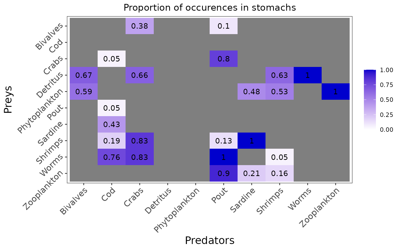
#> Warning: Use of `biotracer_data$group` is discouraged.
#> ℹ Use `group` instead.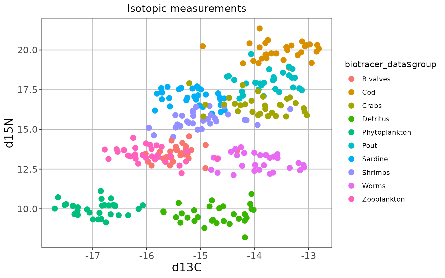
Yes, we are aware that isotopic data is usually messier, but isn’t it a beautiful plot?
The configuration without literature data
We define the configuration we are in, and preprocess the data:
literature_configuration <- FALSE

data <- preprocess_data(biotracer_data = realistic_biotracer_data,
                        trophic_discrimination_factor = c(0.8, 3.4),
                        literature_configuration = literature_configuration,
                        stomach_data = realistic_stomach_data)
#> The model will investigate the following trophic links:
#>               Bivalves Cod Crabs Detritus Phytoplankton Pout Sardine Shrimps
#> Bivalves             0   0     1        0             0    1       0       0
#> Cod                  0   0     0        0             0    0       0       0
#> Crabs                0   1     0        0             0    1       0       0
#> Detritus             1   0     1        0             0    0       0       1
#> Phytoplankton        1   0     0        0             0    0       1       1
#> Pout                 0   1     0        0             0    0       0       0
#> Sardine              0   1     0        0             0    0       0       0
#> Shrimps              0   1     1        0             0    1       1       0
#> Worms                0   1     1        0             0    1       0       1
#> Zooplankton          0   0     0        0             0    1       1       1
#>               Worms Zooplankton
#> Bivalves          0           0
#> Cod               0           0
#> Crabs             0           0
#> Detritus          1           0
#> Phytoplankton     0           1
#> Pout              0           0
#> Sardine           0           0
#> Shrimps           0           0
#> Worms             0           0
#> Zooplankton       0           0
In this configuration, priors are set for each trophic link identified as plausible by the user but the priors are not informed by literature data, and are thus uninformative:
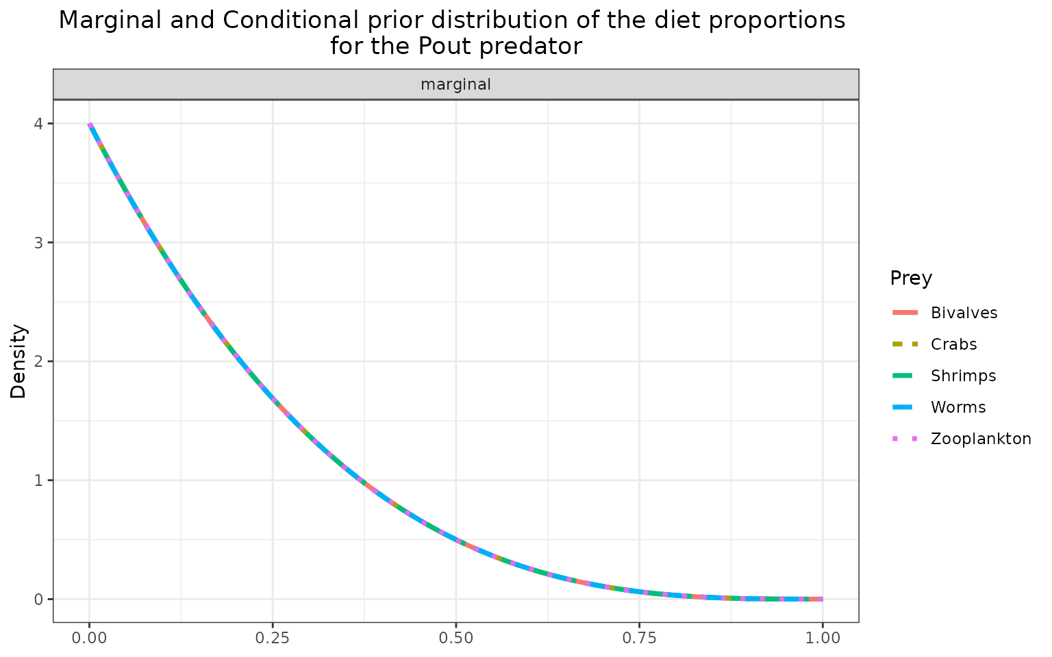
plot_prior(data, literature_configuration)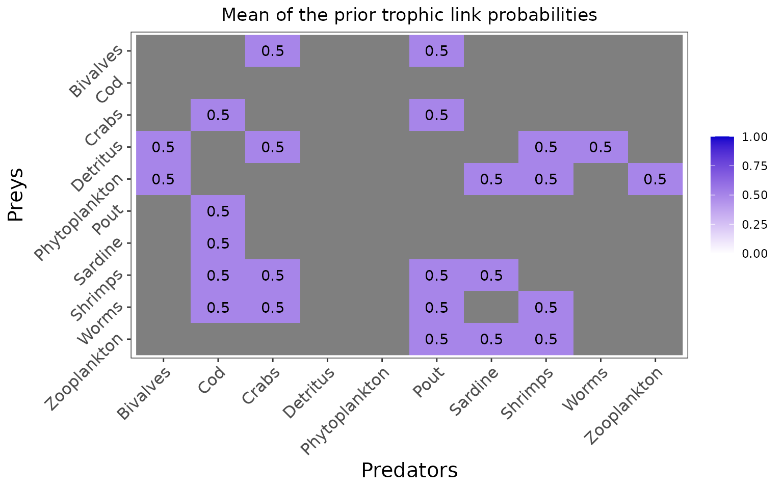
The marginal prior distributions have different shape depending on the variables:
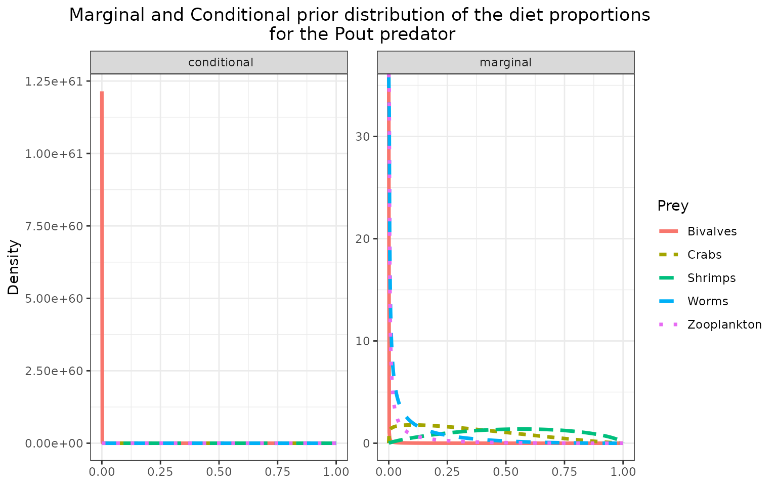
it is flat or uniform for \(\eta\), the probabilities that a trophic link exists (all the probabilities of existence are thus equiprobable),
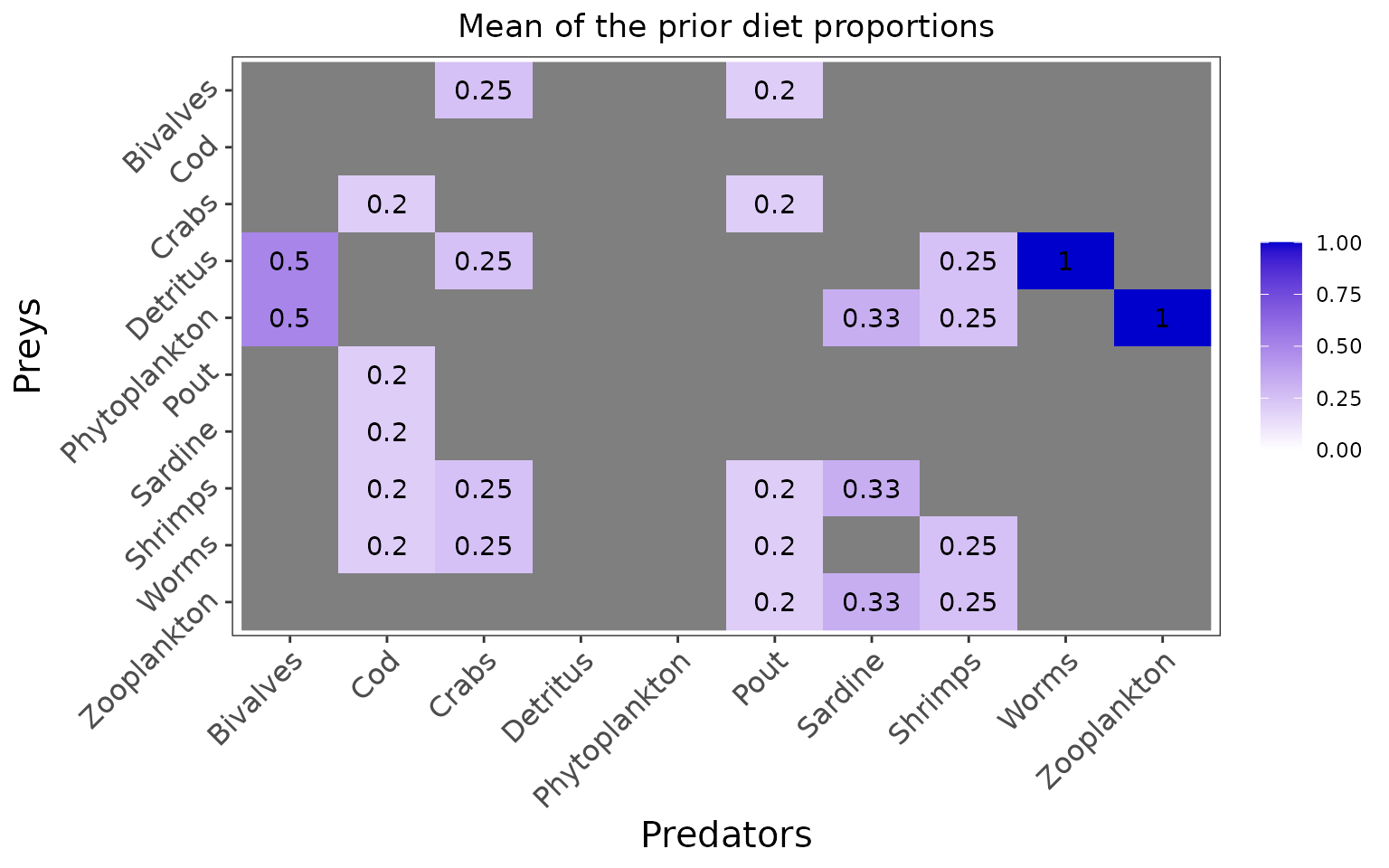
the marginal distributions for each diet proportion \(\Pi\) are peaking at zero, although the joint distribution for \(\Pi\)s is a flat Dirichlet prior, because all the diet proportions must sum to one.
plot_prior(data, literature_configuration, pred = "Pout")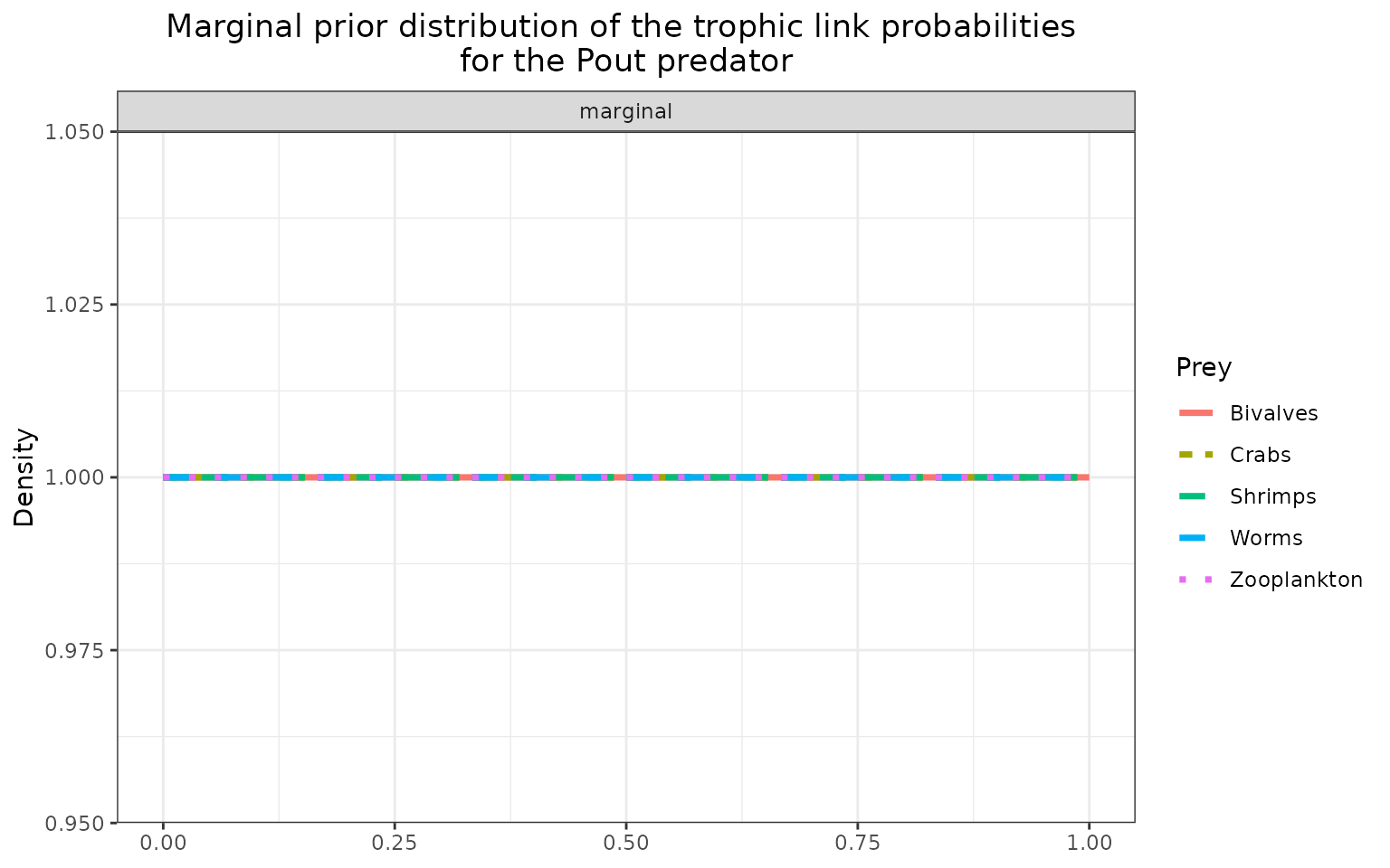
We define the model, and test if it compiles well with a few iterations and adaptation steps:
filename <- "mymodel.txt"
write_model(file.name = filename, literature_configuration = literature_configuration, print.model = F)
mcmc_output <- run_model(filename, data, run_param="test")
#>
#> Processing function input.......
#>
#> Done.
#>
#> Compiling model graph
#>    Resolving undeclared variables
#>    Allocating nodes
#> Graph information:
#>    Observed stochastic nodes: 316
#>    Unobserved stochastic nodes: 125
#>    Total graph size: 1104
#>
#> Initializing model
#>
#> Adaptive phase, 500 iterations x 3 chains
#> If no progress bar appears JAGS has decided not to adapt
#>
#>
#>  Burn-in phase, 500 iterations x 3 chains
#>
#>
#> Sampling from joint posterior, 500 iterations x 3 chains
#>
#>
#> Calculating statistics.......
#>
#> Done.
#>
#>   /!\ Convergence warning:
#> Out of the 51 variables, 14 variables have a Gelman-Rubin statistic > 1.1.
#> You may consider modifying the model run settings.
#> The variables with the poorest convergence are: PI[4,3], PI[10,8], PI[10,7], PI[8,6], PI[8,2], PI[6,2], PI[7,2], PI[9,8], PI[9,3], PI[8,7].
#> JAGS output for model 'mymodel.txt', generated by jagsUI.
#> Estimates based on 3 chains of 1000 iterations,
#> adaptation = 500 iterations (sufficient),
#> burn-in = 500 iterations and thin rate = 1,
#> yielding 1500 total samples from the joint posterior.
#> MCMC ran for 0.235 minutes at time 2024-07-10 10:08:16.119673.
#>
#>              mean     sd    2.5%     50%   97.5% overlap0 f  Rhat n.eff
#> eta[4,1]    0.648  0.084   0.481   0.648   0.800    FALSE 1 1.002   649
#> eta[5,1]    0.592  0.086   0.419   0.593   0.756    FALSE 1 1.001  1500
#> eta[3,2]    0.091  0.059   0.012   0.080   0.233    FALSE 1 1.000  1500
#> eta[6,2]    0.088  0.059   0.012   0.076   0.240    FALSE 1 1.011   200
#> eta[7,2]    0.425  0.101   0.233   0.425   0.624    FALSE 1 1.002   877
#> eta[8,2]    0.220  0.085   0.082   0.213   0.403    FALSE 1 1.013   153
#> eta[9,2]    0.734  0.092   0.536   0.742   0.888    FALSE 1 1.000  1500
#> eta[1,3]    0.389  0.087   0.225   0.384   0.565    FALSE 1 1.005   449
#> eta[4,3]    0.639  0.085   0.467   0.641   0.801    FALSE 1 1.019   107
#> eta[8,3]    0.808  0.069   0.664   0.813   0.924    FALSE 1 1.000  1500
#> eta[9,3]    0.811  0.069   0.657   0.819   0.927    FALSE 1 0.999  1500
#> eta[1,6]    0.126  0.058   0.036   0.119   0.257    FALSE 1 1.011   241
#> eta[3,6]    0.788  0.070   0.638   0.793   0.908    FALSE 1 1.000  1500
#> eta[8,6]    0.156  0.062   0.054   0.151   0.293    FALSE 1 1.005   404
#> eta[9,6]    0.969  0.029   0.893   0.978   0.999    FALSE 1 1.002  1385
#> eta[10,6]   0.876  0.056   0.751   0.884   0.963    FALSE 1 1.001  1500
#> eta[5,7]    0.491  0.087   0.335   0.487   0.667    FALSE 1 1.001  1161
#> eta[8,7]    0.970  0.029   0.893   0.979   0.999    FALSE 1 1.001  1500
#> eta[10,7]   0.225  0.076   0.096   0.220   0.379    FALSE 1 1.007   289
#> eta[4,8]    0.608  0.108   0.393   0.611   0.810    FALSE 1 1.000  1500
#> eta[5,8]    0.525  0.107   0.314   0.525   0.726    FALSE 1 1.003   540
#> eta[9,8]    0.100  0.065   0.014   0.089   0.251    FALSE 1 1.002   666
#> eta[10,8]   0.194  0.083   0.062   0.183   0.370    FALSE 1 1.005   384
#> eta[4,9]    0.948  0.050   0.815   0.964   0.998    FALSE 1 1.001  1034
#> eta[5,10]   0.953  0.045   0.836   0.967   0.999    FALSE 1 1.005   516
#> PI[4,1]     0.394  0.286   0.000   0.361   0.966    FALSE 1 1.014   138
#> PI[5,1]     0.606  0.286   0.034   0.639   1.000    FALSE 1 1.014   138
#> PI[3,2]     0.217  0.296   0.000   0.053   0.951    FALSE 1 1.059    60
#> PI[6,2]     0.167  0.231   0.000   0.024   0.766    FALSE 1 1.460     8
#> PI[7,2]     0.122  0.210   0.000   0.000   0.718    FALSE 1 1.364    11
#> PI[8,2]     0.284  0.335   0.000   0.124   0.998    FALSE 1 1.489     8
#> PI[9,2]     0.209  0.204   0.000   0.152   0.770    FALSE 1 1.032   281
#> PI[1,3]     0.163  0.232   0.000   0.040   0.795    FALSE 1 1.208    17
#> PI[4,3]     0.163  0.202   0.000   0.000   0.583    FALSE 1 2.878     4
#> PI[8,3]     0.277  0.210   0.000   0.253   0.719    FALSE 1 1.050    66
#> PI[9,3]     0.397  0.305   0.002   0.330   0.997    FALSE 1 1.291    11
#> PI[1,6]     0.069  0.133   0.000   0.001   0.493    FALSE 1 1.239    15
#> PI[3,6]     0.320  0.193   0.011   0.304   0.741    FALSE 1 1.069    36
#> PI[8,6]     0.051  0.120   0.000   0.001   0.467    FALSE 1 1.520    10
#> PI[9,6]     0.291  0.200   0.011   0.258   0.732    FALSE 1 1.003  1429
#> PI[10,6]    0.269  0.192   0.005   0.239   0.708    FALSE 1 1.033    75
#> PI[5,7]     0.328  0.180   0.000   0.340   0.653    FALSE 1 1.147    24
#> PI[8,7]     0.578  0.196   0.101   0.602   0.905    FALSE 1 1.279    13
#> PI[10,7]    0.094  0.234   0.000   0.000   0.882    FALSE 1 1.705     7
#> PI[4,8]     0.213  0.206   0.000   0.159   0.728    FALSE 1 1.021   143
#> PI[5,8]     0.301  0.216   0.001   0.283   0.777    FALSE 1 1.185    15
#> PI[9,8]     0.219  0.191   0.000   0.162   0.642    FALSE 1 1.331    10
#> PI[10,8]    0.266  0.271   0.000   0.169   0.857    FALSE 1 1.770     6
#> PI[4,9]     1.000  0.000   1.000   1.000   1.000    FALSE 1    NA     1
#> PI[5,10]    1.000  0.000   1.000   1.000   1.000    FALSE 1    NA     1
#> deviance  866.400 11.003 846.223 865.943 887.645    FALSE 1 1.019   106
#>
#> **WARNING** Some Rhat values could not be calculated.
#> **WARNING** Rhat values indicate convergence failure.
#> Rhat is the potential scale reduction factor (at convergence, Rhat=1).
#> For each parameter, n.eff is a crude measure of effective sample size.
#>
#> overlap0 checks if 0 falls in the parameter's 95% credible interval.
#> f is the proportion of the posterior with the same sign as the mean;
#> i.e., our confidence that the parameter is positive or negative.
#>
#> DIC info: (pD = var(deviance)/2)
#> pD = 59.5 and DIC = 925.854
#> DIC is an estimate of expected predictive error (lower is better).
You should now try to run the model until it converges (it should take around half an hour to run, so we won’t do it in this vignette):
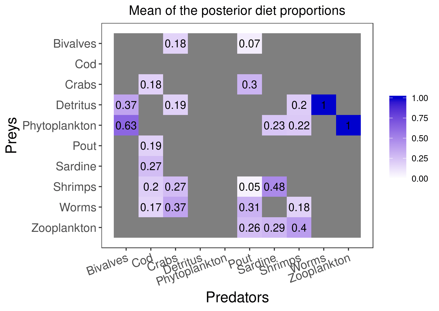
mcmc_output <- run_model(filename, data, run_param="normal", parallelize = T)Here are the figures corresponding to the results that have converged:
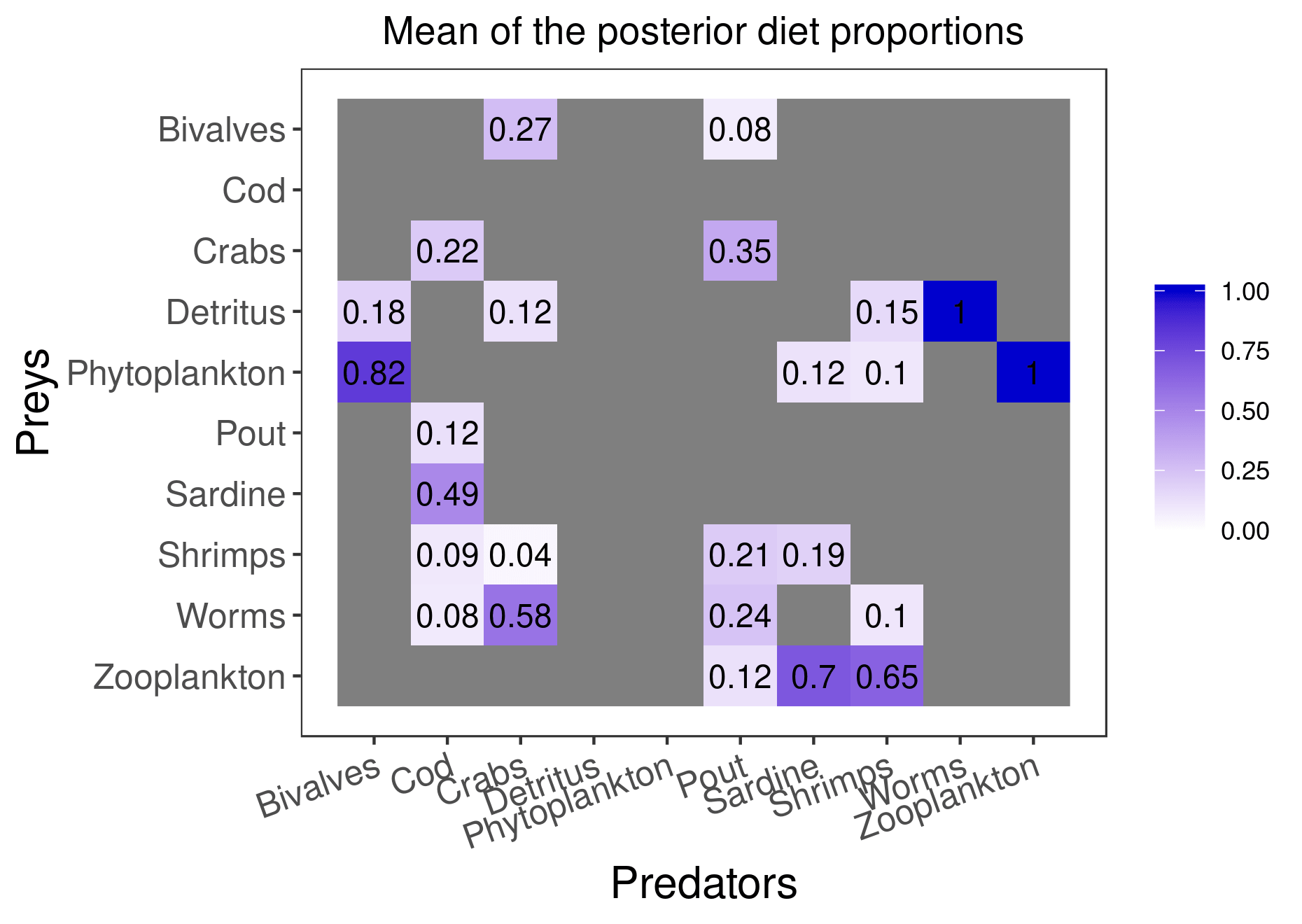
plot_results(mcmc_output, data)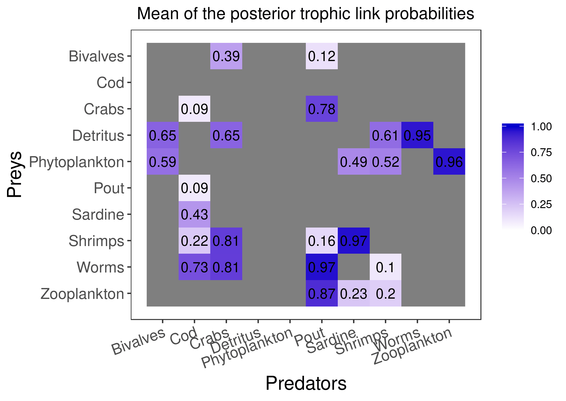
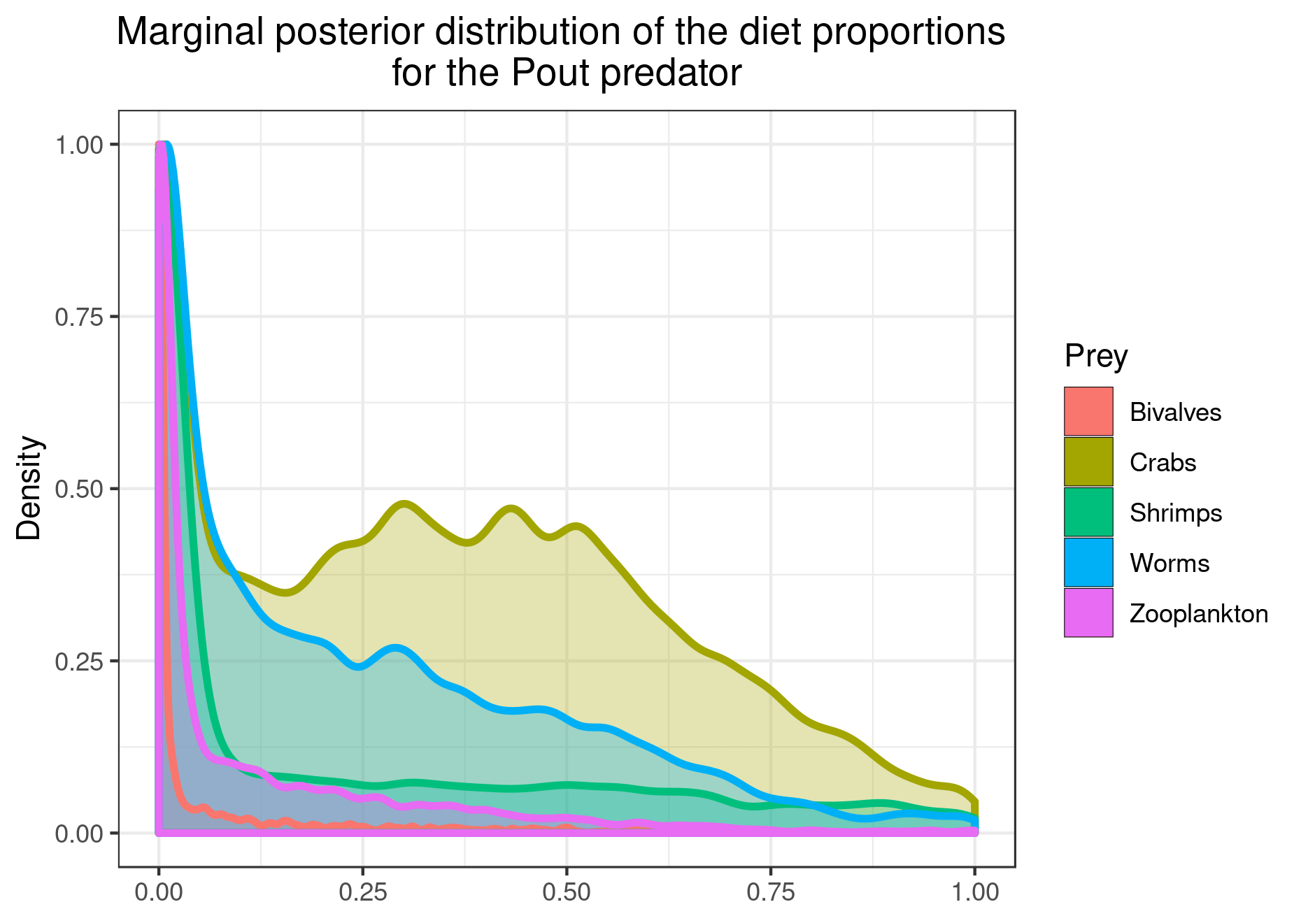
plot_results(mcmc_output, data, pred = "Pout")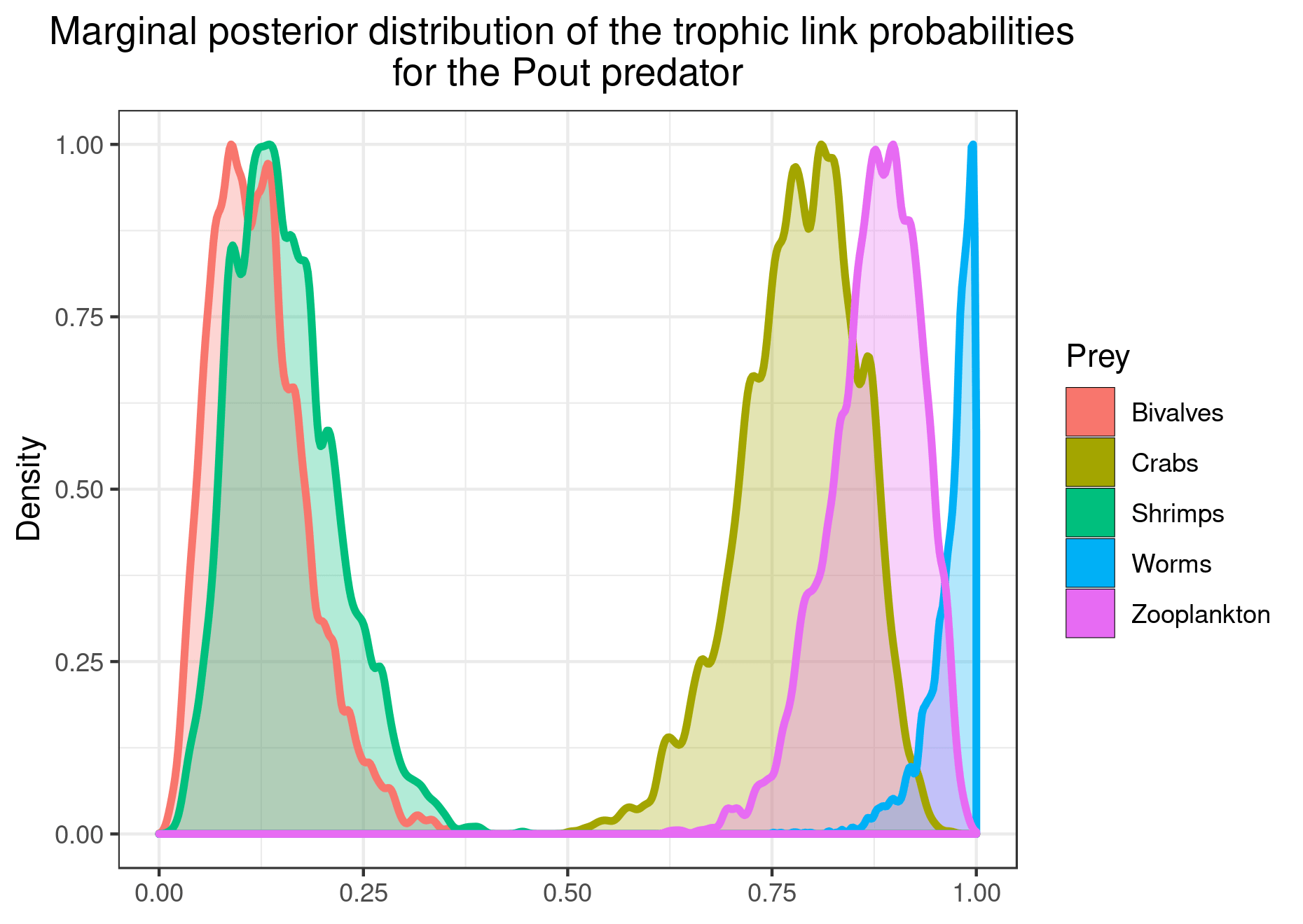
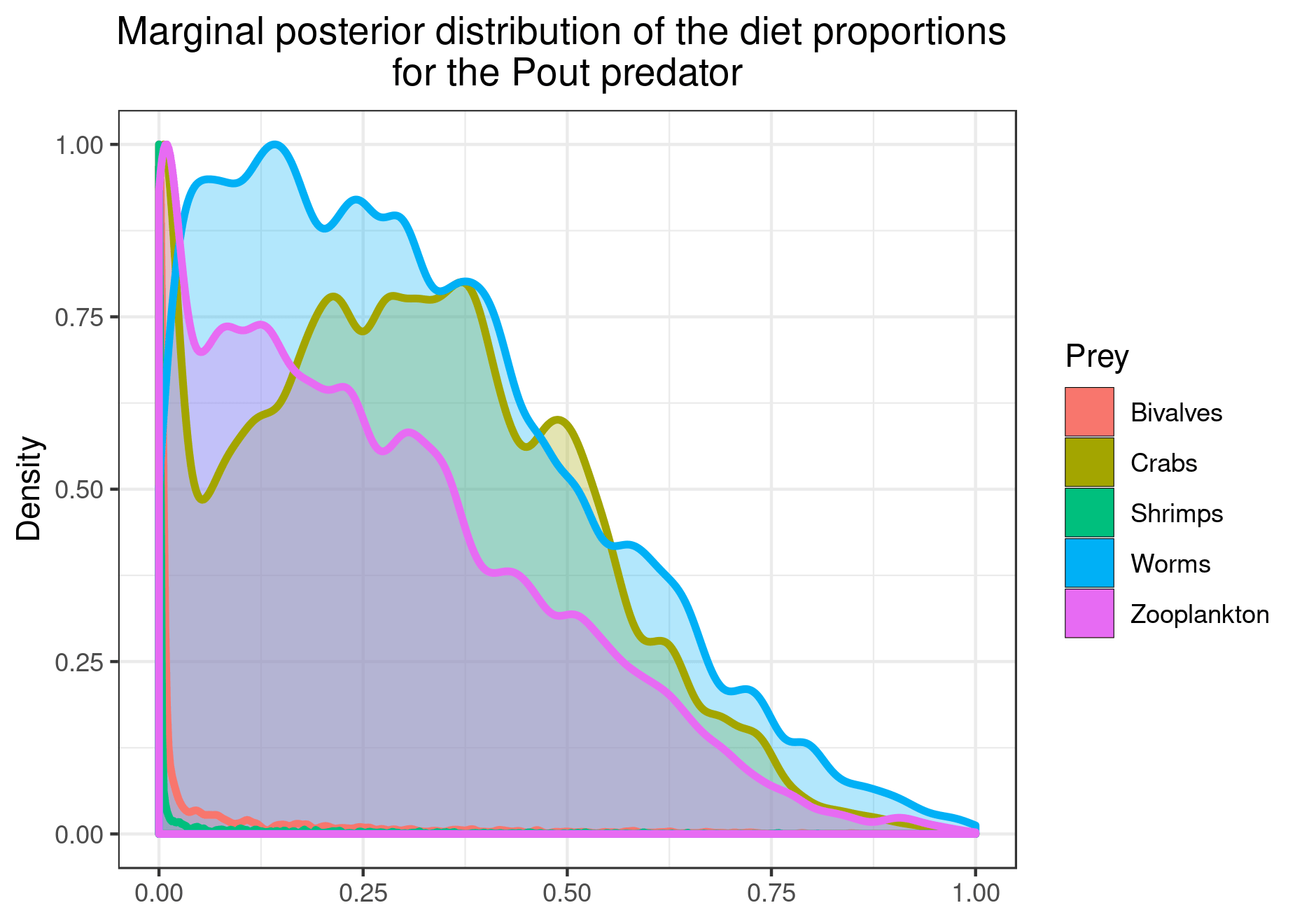
You can also plot the results for specific prey if you want a clearer figure:
plot_results(mcmc_output, data, pred = "Pout",
             variable = "PI", prey = c("Bivalves", "Worms"))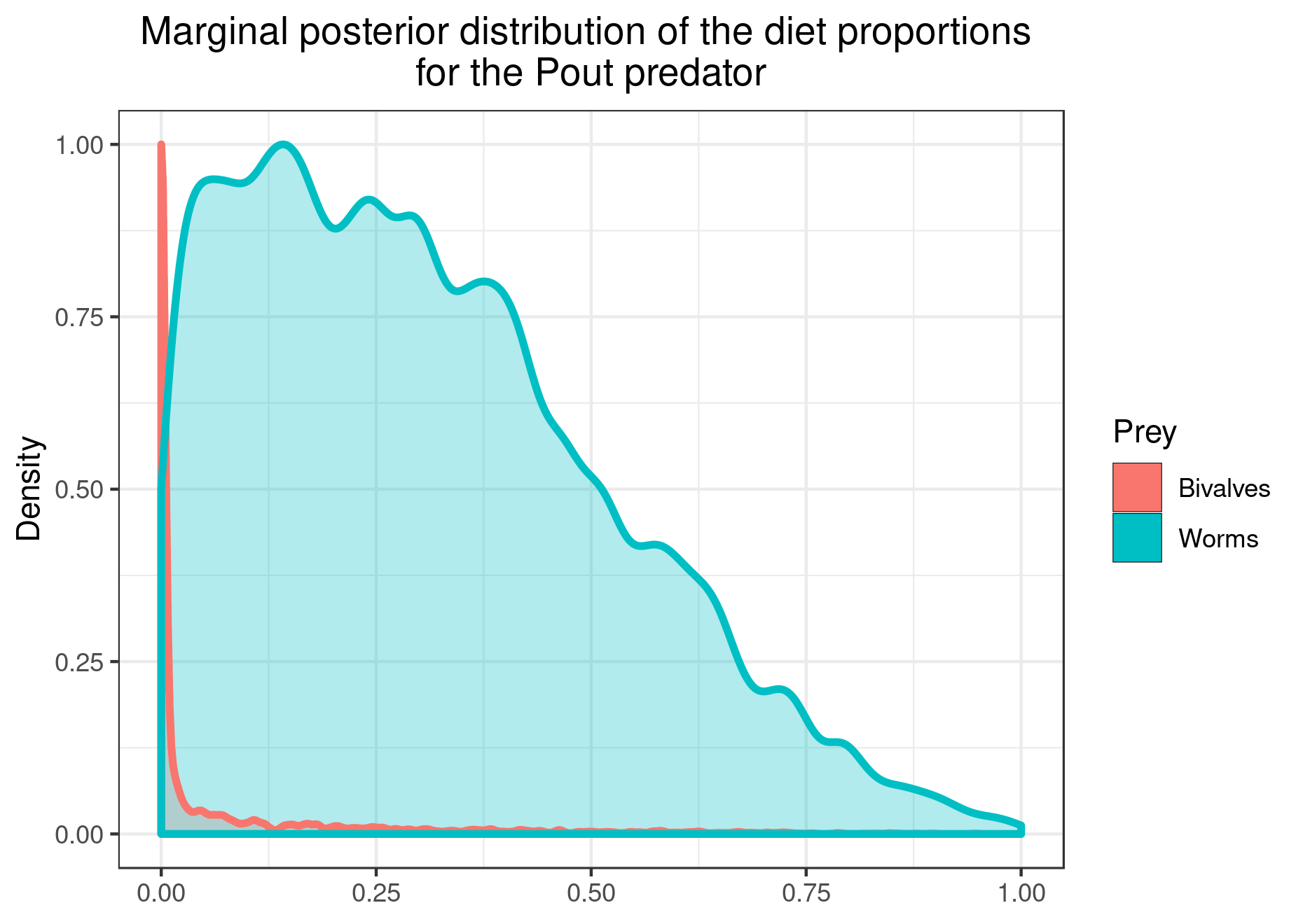
The configuration with literature data
We now change the configuration to add literature data to the model:
literature_configuration <- TRUE
realistic_literature_diets_path <- system.file("extdata", "realistic_literature_diets.csv",
                                               package = "EcoDiet")
realistic_literature_diets <- read.csv(realistic_literature_diets_path)
knitr::kable(realistic_literature_diets)| X | Cod | Pout | Sardine | Shrimps | Crabs | Bivalves | Worms | Zooplankton | Phytoplankton | Detritus |
|---|---|---|---|---|---|---|---|---|---|---|
| Cod | 0.0000000 | 0.0000000 | 0.0000000 | 0.0000000 | 0.0000000 | 0.0000000 | 0.0 | 0.0 | 0 | 0 |
| Pout | 0.4275065 | 0.0000000 | 0.0000000 | 0.0000000 | 0.0000000 | 0.0000000 | 0.0 | 0.0 | 0 | 0 |
| Sardine | 0.3603675 | 0.0000000 | 0.0000000 | 0.0000000 | 0.0000000 | 0.0000000 | 0.0 | 0.0 | 0 | 0 |
| Shrimps | 0.0300737 | 0.5295859 | 0.0002143 | 0.0000000 | 0.0082107 | 0.0000000 | 0.0 | 0.0 | 0 | 0 |
| Crabs | 0.1410430 | 0.3332779 | 0.0000000 | 0.0000000 | 0.0000000 | 0.0000000 | 0.0 | 0.0 | 0 | 0 |
| Bivalves | 0.0000000 | 0.0006130 | 0.0000000 | 0.0000000 | 0.3441081 | 0.0000000 | 0.0 | 0.0 | 0 | 0 |
| Worms | 0.0410093 | 0.1023676 | 0.0000000 | 0.0171336 | 0.4435377 | 0.0000000 | 0.0 | 0.0 | 0 | 0 |
| Zooplankton | 0.0000000 | 0.0341557 | 0.7381375 | 0.9121505 | 0.0000000 | 0.0000000 | 0.0 | 0.0 | 0 | 0 |
| Phytoplankton | 0.0000000 | 0.0000000 | 0.2616482 | 0.0000610 | 0.0000000 | 0.9966847 | 0.0 | 1.0 | 0 | 0 |
| Detritus | 0.0000000 | 0.0000000 | 0.0000000 | 0.0706550 | 0.2041434 | 0.0033153 | 1.0 | 0.0 | 0 | 0 |
| pedigree | 0.8000000 | 0.1000000 | 0.5000000 | 0.3000000 | 0.7000000 | 0.1000000 | 0.2 | 0.2 | 1 | 1 |
data <- preprocess_data(biotracer_data = realistic_biotracer_data,
trophic_discrimination_factor = c(0.8, 3.4),
literature_configuration = literature_configuration,
stomach_data = realistic_stomach_data,
literature_diets = realistic_literature_diets,
nb_literature = 12,
literature_slope = 0.5)
#> The model will investigate the following trophic links:
#> Bivalves Cod Crabs Detritus Phytoplankton Pout Sardine Shrimps
#> Bivalves 0 0 1 0 0 1 0 0
#> Cod 0 0 0 0 0 0 0 0
#> Crabs 0 1 0 0 0 1 0 0
#> Detritus 1 0 1 0 0 0 0 1
#> Phytoplankton 1 0 0 0 0 0 1 1
#> Pout 0 1 0 0 0 0 0 0
#> Sardine 0 1 0 0 0 0 0 0
#> Shrimps 0 1 1 0 0 1 1 0
#> Worms 0 1 1 0 0 1 0 1
#> Zooplankton 0 0 0 0 0 1 1 1
#> Worms Zooplankton
#> Bivalves 0 0
#> Cod 0 0
#> Crabs 0 0
#> Detritus 1 0
#> Phytoplankton 0 1
#> Pout 0 0
#> Sardine 0 0
#> Shrimps 0 0
#> Worms 0 0
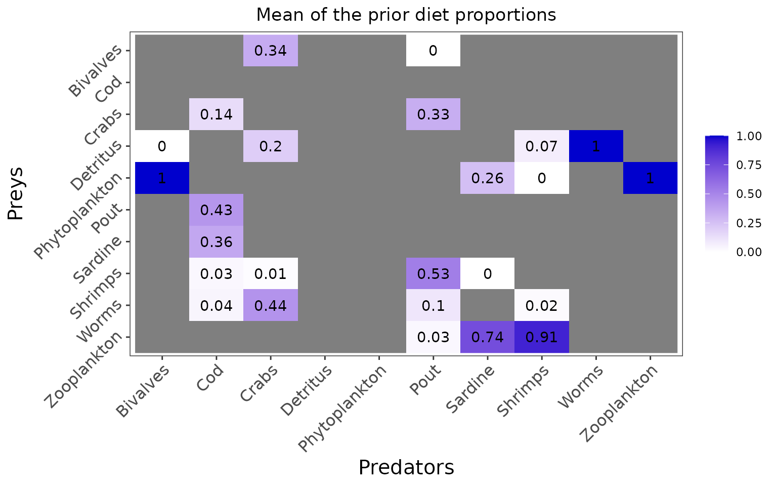
#> Zooplankton 0 0Now we see that the prior distributions are informed by the literature data:
when the literature diet input is > 0, the trophic link probabilities \(\eta\) are shifted toward one. Here this is the case for all prey but we could imagine that the user identify a species as a plausible prey whereas it has not been observed being consumed by the predator in the literature. In that case, the literature diet of 0 would drive \(\eta\) toward 0.
the average prior for the diet proportions \(\Pi\) is directly the literature diet input.
plot_prior(data, literature_configuration)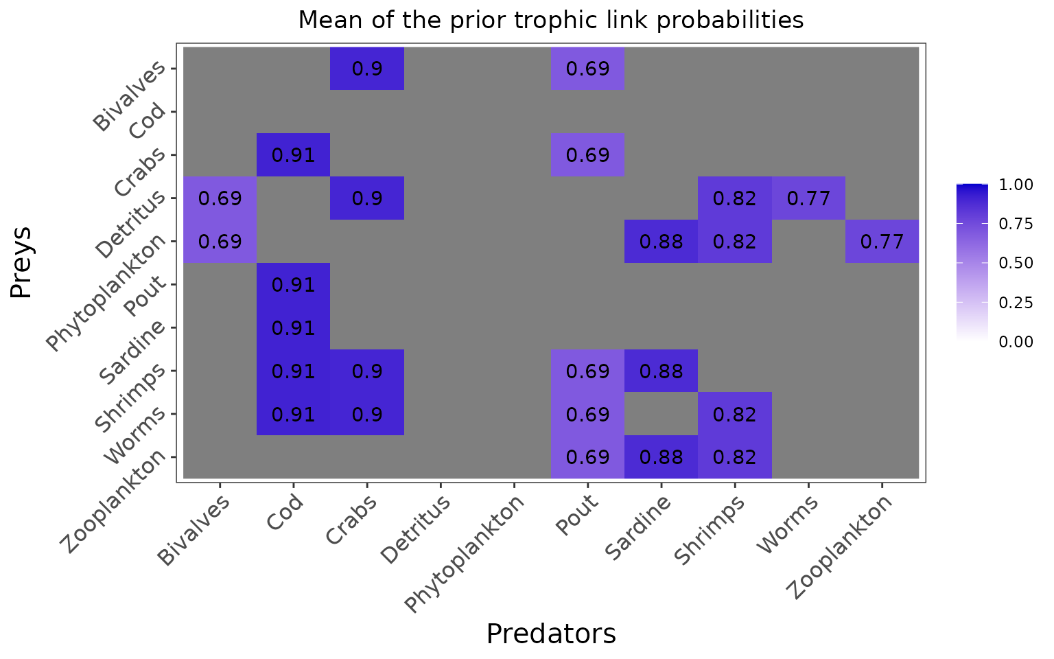
plot_prior(data, literature_configuration, pred = "Pout")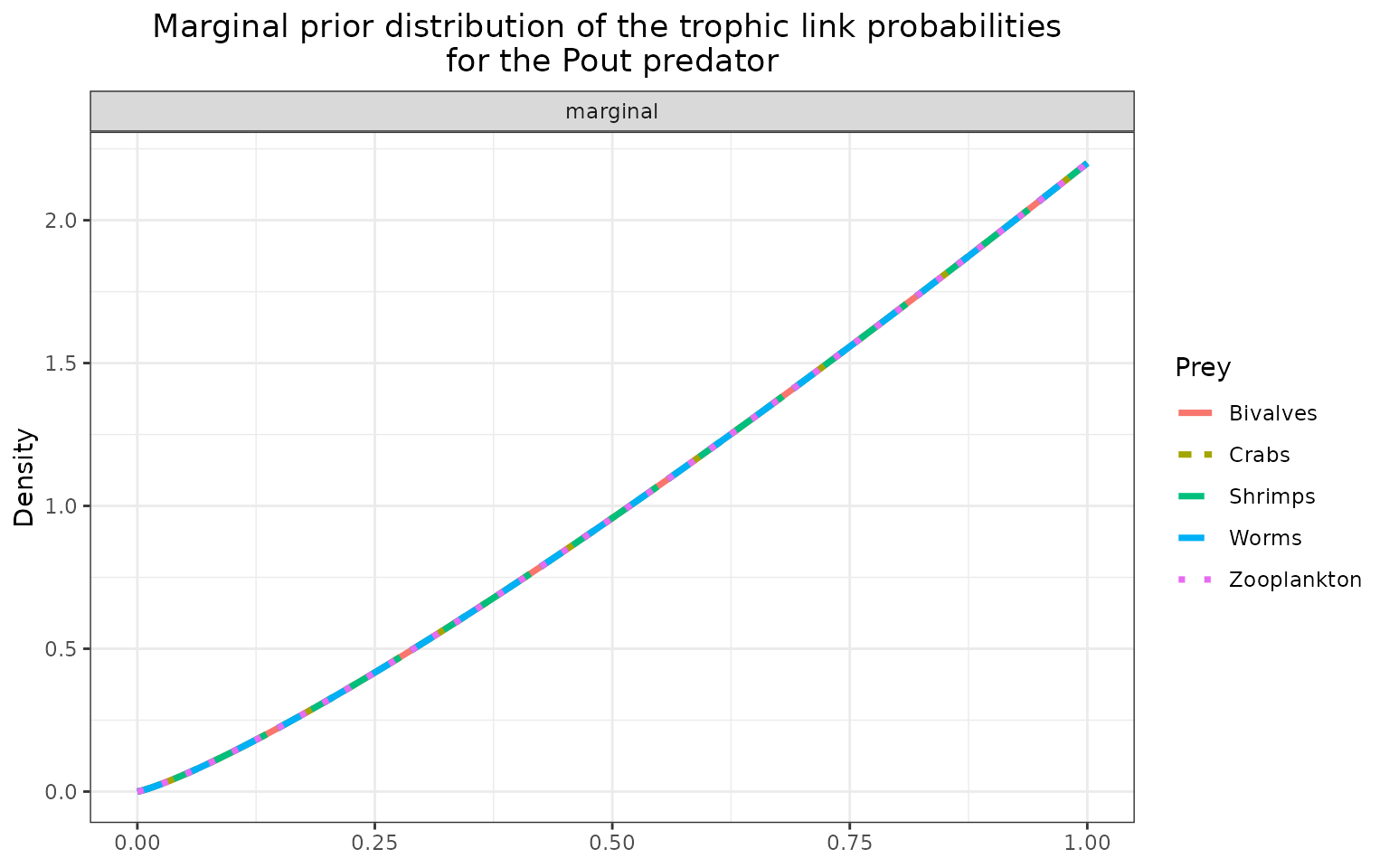
Again, we verify that the model compiles well:
filename <- "mymodel_literature.txt"
write_model(file.name = filename, literature_configuration = literature_configuration, print.model = F)
mcmc_output <- run_model(filename, data, run_param="test")
#>
#> Processing function input.......
#>
#> Done.
#>
#> Compiling model graph
#>    Resolving undeclared variables
#>    Allocating nodes
#> Graph information:
#>    Observed stochastic nodes: 316
#>    Unobserved stochastic nodes: 125
#>    Total graph size: 1594
#>
#> Initializing model
#>
#> Adaptive phase, 500 iterations x 3 chains
#> If no progress bar appears JAGS has decided not to adapt
#>
#>
#>  Burn-in phase, 500 iterations x 3 chains
#>
#>
#> Sampling from joint posterior, 500 iterations x 3 chains
#>
#>
#> Calculating statistics.......
#>
#> Done.
#>
#>   /!\ Convergence warning:
#> Out of the 51 variables, 17 variables have a Gelman-Rubin statistic > 1.1.
#> You may consider modifying the model run settings.
#> The variables with the poorest convergence are: PI[10,7], PI[8,7], PI[5,7], PI[7,2], PI[10,8], PI[6,2], PI[1,6], PI[3,2], PI[1,3], PI[9,8].
#> JAGS output for model 'mymodel_literature.txt', generated by jagsUI.
#> Estimates based on 3 chains of 1000 iterations,
#> adaptation = 500 iterations (sufficient),
#> burn-in = 500 iterations and thin rate = 1,
#> yielding 1500 total samples from the joint posterior.
#> MCMC ran for 0.234 minutes at time 2024-07-10 10:08:34.460153.
#>
#>              mean     sd    2.5%     50%   97.5% overlap0 f  Rhat n.eff
#> eta[4,1]    0.663  0.085   0.499   0.666   0.822    FALSE 1 1.002   834
#> eta[5,1]    0.609  0.087   0.430   0.611   0.772    FALSE 1 0.999  1500
#> eta[3,2]    0.366  0.085   0.209   0.365   0.533    FALSE 1 1.003   701
#> eta[6,2]    0.345  0.079   0.203   0.343   0.507    FALSE 1 1.000  1500
#> eta[7,2]    0.599  0.087   0.417   0.601   0.762    FALSE 1 1.013   161
#> eta[8,2]    0.456  0.085   0.289   0.456   0.623    FALSE 1 1.001  1500
#> eta[9,2]    0.815  0.069   0.665   0.822   0.928    FALSE 1 1.000  1500
#> eta[1,3]    0.517  0.078   0.361   0.518   0.661    FALSE 1 1.017   115
#> eta[4,3]    0.719  0.070   0.576   0.723   0.844    FALSE 1 1.001  1500
#> eta[8,3]    0.845  0.055   0.726   0.851   0.937    FALSE 1 1.004   752
#> eta[9,3]    0.851  0.055   0.727   0.857   0.943    FALSE 1 1.000  1500
#> eta[1,6]    0.159  0.064   0.056   0.150   0.310    FALSE 1 1.000  1500
#> eta[3,6]    0.790  0.069   0.649   0.796   0.908    FALSE 1 1.007   273
#> eta[8,6]    0.186  0.067   0.074   0.181   0.334    FALSE 1 1.004   540
#> eta[9,6]    0.970  0.028   0.895   0.978   0.999    FALSE 1 1.000  1500
#> eta[10,6]   0.880  0.057   0.749   0.887   0.967    FALSE 1 1.001  1500
#> eta[5,7]    0.563  0.081   0.395   0.565   0.711    FALSE 1 1.000  1500
#> eta[8,7]    0.974  0.026   0.896   0.982   0.999    FALSE 1 1.000  1500
#> eta[10,7]   0.358  0.077   0.215   0.355   0.507    FALSE 1 1.038    59
#> eta[4,8]    0.675  0.093   0.487   0.678   0.841    FALSE 1 1.002   803
#> eta[5,8]    0.595  0.096   0.408   0.601   0.780    FALSE 1 1.000  1500
#> eta[9,8]    0.234  0.086   0.088   0.228   0.420    FALSE 1 1.003   637
#> eta[10,8]   0.305  0.092   0.141   0.300   0.496    FALSE 1 1.001  1500
#> eta[4,9]    0.957  0.042   0.843   0.970   0.999    FALSE 1 1.006  1500
#> eta[5,10]   0.958  0.039   0.846   0.969   0.999    FALSE 1 1.002   850
#> PI[4,1]     0.097  0.209   0.000   0.000   0.810    FALSE 1 1.173    23
#> PI[5,1]     0.903  0.209   0.190   1.000   1.000    FALSE 1 1.173    23
#> PI[3,2]     0.402  0.336   0.000   0.341   0.996    FALSE 1 1.307    11
#> PI[6,2]     0.042  0.133   0.000   0.000   0.538    FALSE 1 1.478    12
#> PI[7,2]     0.302  0.323   0.000   0.173   0.901    FALSE 1 1.843     5
#> PI[8,2]     0.155  0.212   0.000   0.058   0.804    FALSE 1 1.120    37
#> PI[9,2]     0.100  0.119   0.000   0.057   0.420    FALSE 1 1.059    70
#> PI[1,3]     0.176  0.230   0.000   0.033   0.720    FALSE 1 1.306    11
#> PI[4,3]     0.099  0.118   0.000   0.054   0.404    FALSE 1 1.016   317
#> PI[8,3]     0.039  0.093   0.000   0.001   0.321    FALSE 1 1.197    27
#> PI[9,3]     0.685  0.244   0.154   0.726   0.998    FALSE 1 1.104    25
#> PI[1,6]     0.127  0.177   0.000   0.030   0.620    FALSE 1 1.405     9
#> PI[3,6]     0.367  0.260   0.000   0.354   0.883    FALSE 1 1.015   290
#> PI[8,6]     0.193  0.273   0.000   0.016   0.872    FALSE 1 1.127    27
#> PI[9,6]     0.279  0.241   0.000   0.237   0.845    FALSE 1 1.084    33
#> PI[10,6]    0.033  0.077   0.000   0.001   0.263    FALSE 1 1.011  1231
#> PI[5,7]     0.155  0.190   0.000   0.062   0.600    FALSE 1 2.029     5
#> PI[8,7]     0.221  0.323   0.000   0.001   0.932    FALSE 1 5.692     3
#> PI[10,7]    0.624  0.450   0.000   0.919   1.000    FALSE 1 8.790     3
#> PI[4,8]     0.202  0.201   0.000   0.150   0.716    FALSE 1 1.121    34
#> PI[5,8]     0.252  0.253   0.000   0.192   0.881    FALSE 1 1.028   213
#> PI[9,8]     0.432  0.283   0.000   0.468   0.959    FALSE 1 1.218    17
#> PI[10,8]    0.114  0.264   0.000   0.000   0.936    FALSE 1 1.592     8
#> PI[4,9]     1.000  0.000   1.000   1.000   1.000    FALSE 1    NA     1
#> PI[5,10]    1.000  0.000   1.000   1.000   1.000    FALSE 1    NA     1
#> deviance  867.503 11.272 846.979 867.214 892.252    FALSE 1 1.002  1500
#>
#> **WARNING** Some Rhat values could not be calculated.
#> **WARNING** Rhat values indicate convergence failure.
#> Rhat is the potential scale reduction factor (at convergence, Rhat=1).
#> For each parameter, n.eff is a crude measure of effective sample size.
#>
#> overlap0 checks if 0 falls in the parameter's 95% credible interval.
#> f is the proportion of the posterior with the same sign as the mean;
#> i.e., our confidence that the parameter is positive or negative.
#>
#> DIC info: (pD = var(deviance)/2)
#> pD = 63.6 and DIC = 931.081
#> DIC is an estimate of expected predictive error (lower is better).
You should now try to run the model until it converges (it should take around half an hour to run, so we won’t do it in this vignette):
mcmc_output <- run_model(filename, data, run_param=list(nb_iter=100000, nb_burnin=50000, nb_thin=50, nb_adapt=50000), parallelize = T)Here are the figures corresponding to the results that have converged:
plot_results(mcmc_output, data)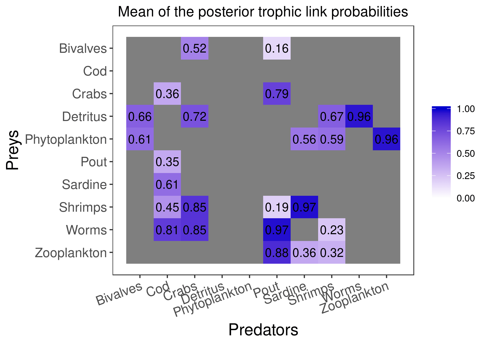
plot_results(mcmc_output, data, pred = "Pout")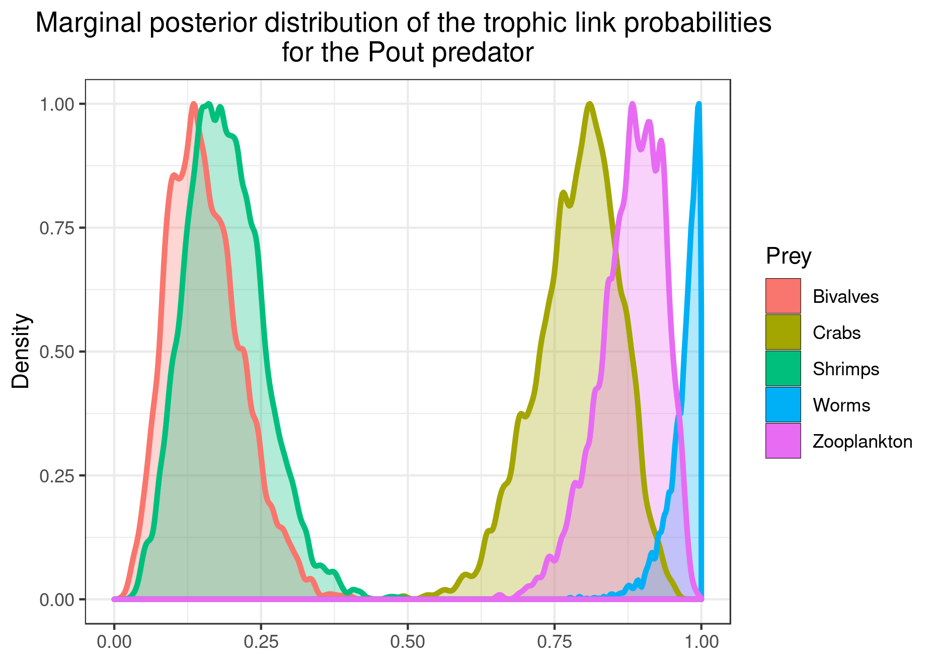
You can save the figures as PNG using:
plot_results(mcmc_output, data, pred = "Pout", save = TRUE, save_path = ".")Last, if you want to explore further in detail the a posteriori distribution of your parameters \(\Pi\) and \(\eta\), you can run the following code line, which will store the values for all iterations into a data frame.
reshape_mcmc(mcmc_output, data)