Density functions

In order to avoid confusion, I will discuss in detail the different ways in which we could describe the size distribution of the stomach items in terms of different density functions.

Prey item distribution

We can describe the size distribution of prey in stomachs of predators of size $w'$ by the number density function $N_w(w|w')$. This is a density in $w$, so that the number of prey items with a size between $w$ and $w+dw$ is $N_w(w|w')dw$.

Alternatively we can describe the size distribution by the probability density that a random prey item in a stomach of a predator of size $w'$ has size $w$. This probability density function is simply the normalised version of the number density: $$f_w(w|w') = \frac{N_w(w|w')}{z(w')},$$ where the normalisation factor $z(w')$ is the total number of prey items, $$z(w') = \int N_w(\tilde{w}|w')d\tilde{w}.$$ The sizes of the actual observed prey items in the data set are seen as samples from this probability distribution.

Rather than working with the prey size $w$, we can also work with the predator/prey mass ratio $r = w' / w$. The probability distribution of this is $$f_r(r|w') = \left|\frac{dw}{dr}\right| f_w(r|w') = \frac{w^2}{w'} f_w(w|w').$$

It is actually a good idea to work with the logarithm of the predator/prey mass ratio $l = \log(r) = \log(w'/w)$. Its distribution is $$f_l(l|w') = \left|\frac{dw}{dl}\right| f_w(w|w') = w f_w(w|w').$$ We will be making the fundamental assumption that the distribution of the predator/prey mass ratio is independent of the predator size: $f_r(r|w') = f_r(r)$ (and hence also $f_l(l|w') = f_l(l)$). Of course we should look at the data to see if this assumption is reasonable.

Biomass distribution

We would also be interested in how the prey biomass is distributed over the prey sizes, because as far as the predator is concerned, it is the amount of biomass that counts, not the number of individuals that are needed to make up that biomass. So instead of the number density $N_w(w|w')$, we would look at the biomass density $B_w(w|w')$, defined so that $B_w(w|w')dw$ is the total biomass of prey items with sizes between $w$ and $w+dw$. The number density and the biomass density are simply related: $$B_w(w|w') = w\ N_w(w|w').$$ Again there is a probability density associated to this: $$b_w(w|w') = \frac{B_w(w|w')}{\int B_w(\tilde{w}|w')d\tilde{w}}.$$ This gives the probability that a randomly chosen unit of biomass in the stomach of a predator of size $w'$ comes from a prey item of size $w$. The relation to the earlier density is $$b_w(w|w') \propto w\ f_w(w|w').$$

To see how this biomass density is related to the observations of stomach contents, consider that instead of recording one observation for each prey individual, we could in principle record one observation for each unit of biomass in the stomach. This would correspond to splitting each single observation for a prey item of size $w$ into $w$ separate observations. This new larger set of observations could then be seen as a sample from the distribution described by the biomass density $b_w(w|w')$.

Again we can transform the probability density to different variables. In particular the density as a function of $l = \log(w'/w)$ is $$b_l(l|w') = w\,b_w(w|w') \propto w^2\,f_w(w|w') \propto w\,f_l(l) \propto e^{-l}f_l(l).$$ So again $b_l(l|w')$ is independent of $w'$.

Transforming densities

We have seen above how the biomass density is obtained from the number density by multiplying by $e^{-l}$ and then normalising again. More generally we might want to transform by multiplying by $e^{-\alpha l}$ for some real number $\alpha$. For the three families of distributions that we are interested in, the normal distribution, the gaussian mixture distribution and the truncated exponential distribution, the miracle is that the transformed density is again a distribution of the same type, just with transformed parameters. We will now derive how the parameters are being transformed.

Normal distribution

If we start with the normal density $$f(l)=\frac{1}{\sqrt{2\pi\sigma^2}}\exp\left(-\frac{(l-\mu)^2}{2\sigma^2}\right)$$ then $$\begin{split} e^{-\alpha l}f(l)&=\frac{1}{\sqrt{2\pi\sigma^2}}\exp\left(-\frac{(l-\mu)^2}{2\sigma^2}-\alpha l\right)\\ &=\frac{1}{\sqrt{2\pi\sigma^2}}\exp\left(-\frac{(l-\mu+\alpha\sigma^2)^2}{2\sigma^2}-\alpha \mu+\frac{\alpha^2}{2}\sigma^2\right)\\ &\propto \frac{1}{\sqrt{2\pi\sigma^2}}\exp\left(-\frac{(l-(\mu-\alpha\sigma^2))^2}{2\sigma^2}\right) \end{split}$$ This can be checked by expanding the square: $$\begin{split} -\frac{(l-(\mu-\alpha\sigma^2))^2}{2\sigma^2} &=-\frac{(l-\mu)^2}{2\sigma^2}-\frac{2l\alpha\sigma^2}{2\sigma^2}+\frac{2\mu\alpha\sigma^2}{2\sigma^2}-\frac{\alpha^2\sigma^4}{2\sigma^2}\\ &=-\frac{(l-\mu)^2}{2\sigma^2}-\alpha l+\alpha\mu-\frac{\alpha^2\sigma^2}{2}. \end{split}$$ So the resulting new distribution has a shifted mean of $\tilde{\mu}=\mu-\alpha\sigma^2$ but the same variance.

Gaussian mixture distribution

Similarly if $f(l)$ is the density of a Gaussian mixture distribution, $$f(l)=\sum_{i=1}^kc_i\frac{1}{\sqrt{2\pi\sigma_i^2}}\exp\left(-\frac{(l-\mu_i)^2}{2\sigma_i^2}\right)$$ then $$\begin{split} e^{-\alpha l}f(l) &=\sum_{i=1}^kc_i\frac{1}{\sqrt{2\pi\sigma_i^2}}\exp\left(-\frac{(l-\mu_i)^2}{2\sigma_i^2}-\alpha l\right)\\ &=\sum_{i=1}^kc_i\frac{1}{\sqrt{2\pi\sigma_i^2}}\exp\left(-\frac{(l-\mu_i+\alpha\sigma_i^2)^2}{2\sigma_i^2}-\alpha \mu_i+\frac{\alpha^2}{2}\sigma_i^2\right)\\ &=\sum_{i=1}^k\left(c_i\exp\left(-\alpha \mu_i+\frac{\alpha^2}{2}\sigma_i^2\right)\right) \frac{1}{\sqrt{2\pi\sigma_i^2}}\exp\left(-\frac{(l-(\mu_i-\alpha\sigma_i^2))^2}{2\sigma_i^2}\right) \end{split}$$ We see that the coefficients of the Gaussians have changed. To get the new normalised distribution we also need to divide by the area under the above density, which is $$\int_{-\infty}^\infty e^{-\alpha l}f(l)dl=\sum_{i=1}^k\left(c_i\exp\left(-\alpha \mu_i+\frac{\alpha^2}{2}\sigma_i^2\right)\right)$$ So $$e^{-\alpha l}f(l)\propto\sum_{i=1}^k\tilde{c}_i\frac{1}{\sqrt{2\pi\sigma_i^2}}\exp\left(-\frac{(l-\tilde{\mu}_i)^2}{2\sigma_i^2}\right)$$ with $$\tilde{\mu}_i=\mu_i-\alpha\sigma_i^2$$ and $$\tilde{c}_i=\frac{\exp\left(-\alpha \mu_i+\frac{\alpha^2}{2}\sigma_i^2\right)} {\sum_{i=1}^kc_i\exp\left(-\alpha \mu_i+\frac{\alpha^2}{2}\sigma_i^2\right)}\,c_i$$

Let us check this analytic result also numerically.

c <- c(0.2, 0.3, 0.5)
mu <- c(3, 4, 6)
sigma <- c(0.2, 0.5, 2)
fl <- function(l, c, mu, sigma) {
    f <- 0
    for (i in seq_along(c)) {
        f <- f + c[i]*dnorm(l, mean = mu[i], sd = sigma[i])
    }
    f
}

l <- seq(0, 15, by = 0.1)
plot(l, fl(l, c, mu, sigma), type = "l", lty = 3, ylab = "Density")

alpha = -1
shifted_fl <- exp(-alpha * l) * fl(l, c, mu, sigma)
shifted_fl <- shifted_fl / sum(shifted_fl * 0.1)
lines(l, shifted_fl, col = "green", lty = 1)

mu_shifted <- mu - alpha * sigma^2
c_shifted <- c * exp(-alpha * mu + alpha^2 / 2 * sigma^2)
c_shifted <- c_shifted / sum(c_shifted)
lines(l, fl(l, c_shifted, mu_shifted, sigma), col = "blue", lty = 2)

legend("topright", legend = c("original", "numerically shifted", "analytically shifted"), 
       col = c("black", "green", "blue"), lty = c(3, 1, 2), cex = 0.8)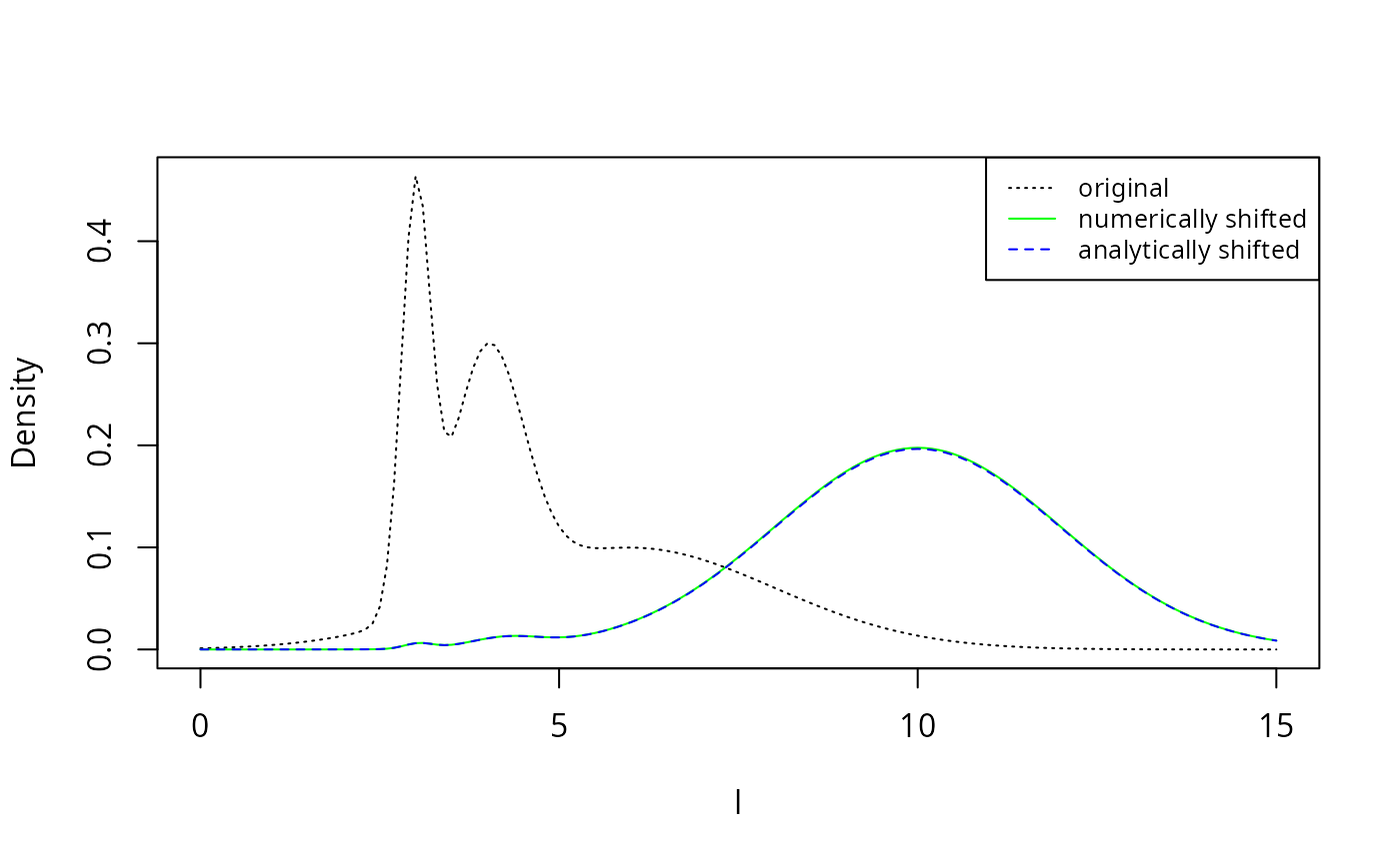

The numerically shifted line in green is perfectly covered by the analytically shifted line in blue, thereby confirming the analytic results above.