Estimating growth rates from age-at-size data

I still need to write this vignette.

library(growthEstimation)
pars <- list(
    k = 0.1,
    L_inf = 110,
    d = 1,
    m = 1,
    annuli_date = 0,
    annuli_min_age = 0,
    spawning_mu = 0.4,
    spawning_kappa = 10
)

age_at_length <- Cod_CS_age_at_length

plotAgeLikelihood(pars, age_at_length)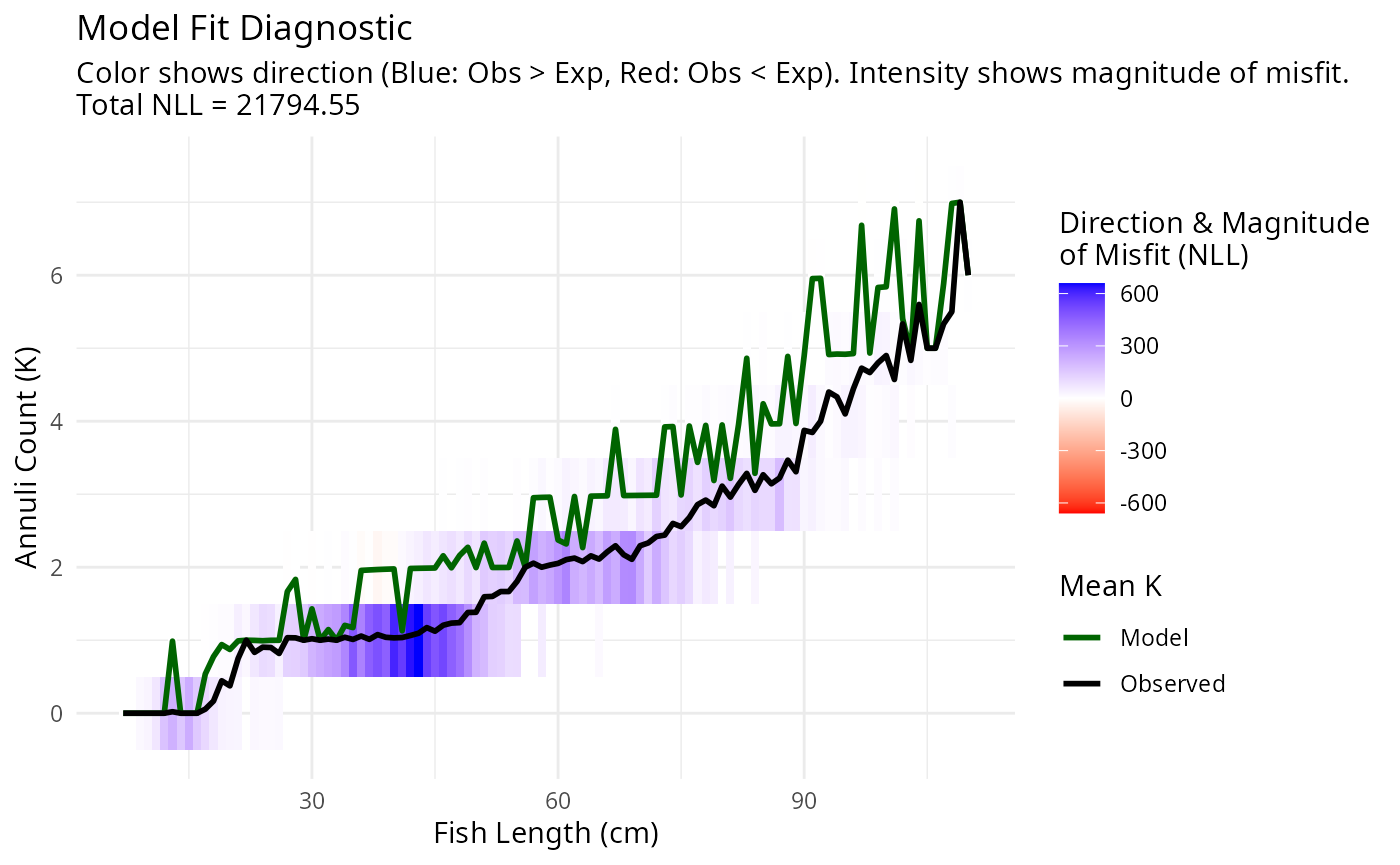

To start tuning parameters, run the following code. A Shiny app will open

tune_pars(pars, age_at_length)

You can automatically tune the parameters with

fit <- fit_tmb_nll(pars, surveys = age_at_length)

pars <- fit$pars
plotAgeLikelihood(pars, age_at_length)

The parameters appear to fit the age-at-size data, but the mortality and diffusion coefficients are too low. The estimated parameters are:

parameter_names <- c("k", "L_inf", "d", "m", "annuli_min_age")
pars[parameter_names]

## $k
## [1] 0.1974143
## 
## $L_inf
## [1] 164.8323
## 
## $d
## [1] 1e-06
## 
## $m
## [1] 1e-06
## 
## $annuli_min_age
## [1] 0

This leads to the following time evolution of a yearly cohort:

u <- getNumberDensity(pars, l_max = 200, t_max = 15)
plotDensity2D(u)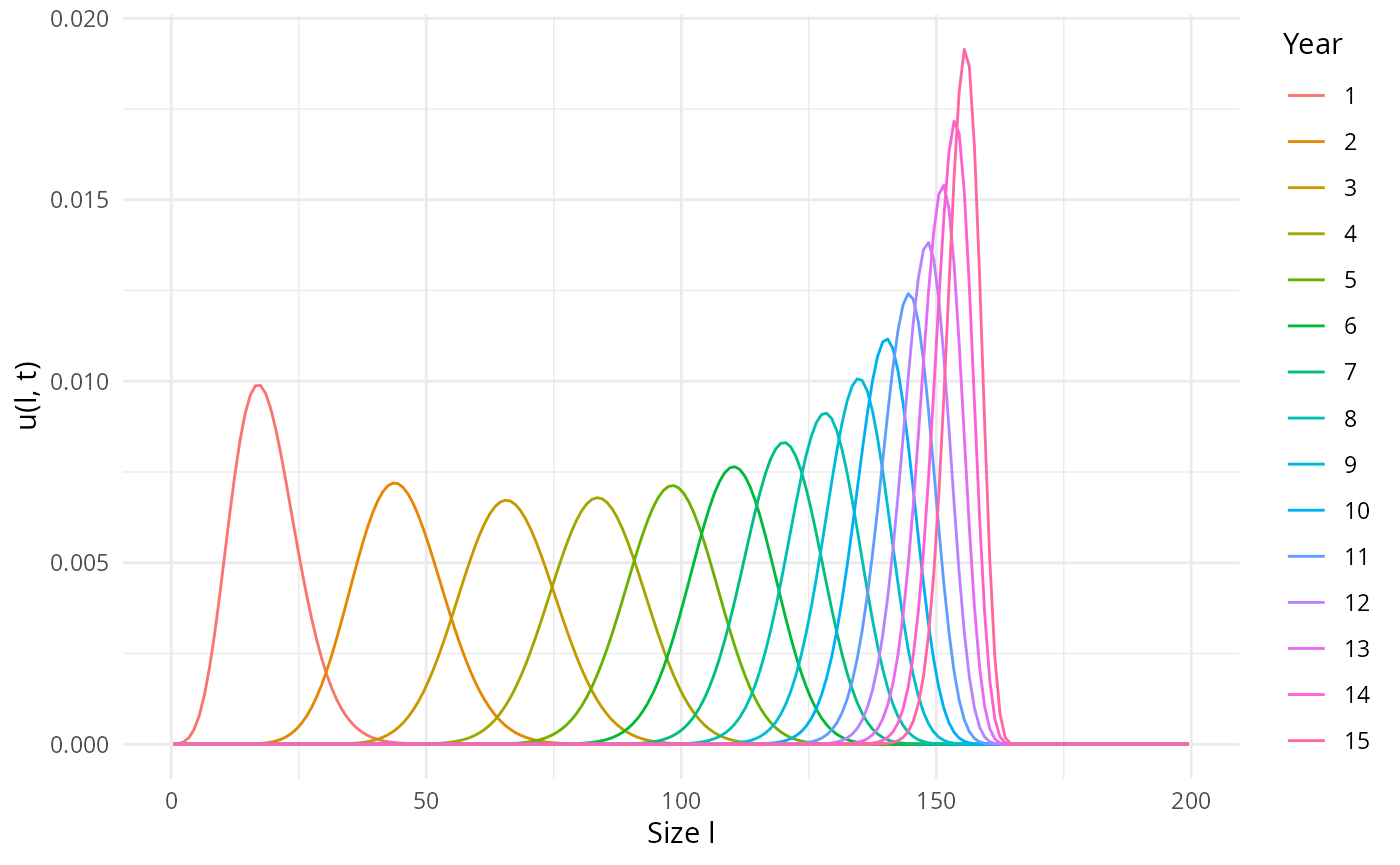

plotDensity3D(u)

If we constrain the mortality coefficient to be at least 30 we get:

fit <- fit_tmb_nll(pars, surveys = age_at_length,
                   lower = c(m = 25))

pars <- fit$pars
plotAgeLikelihood(pars, age_at_length)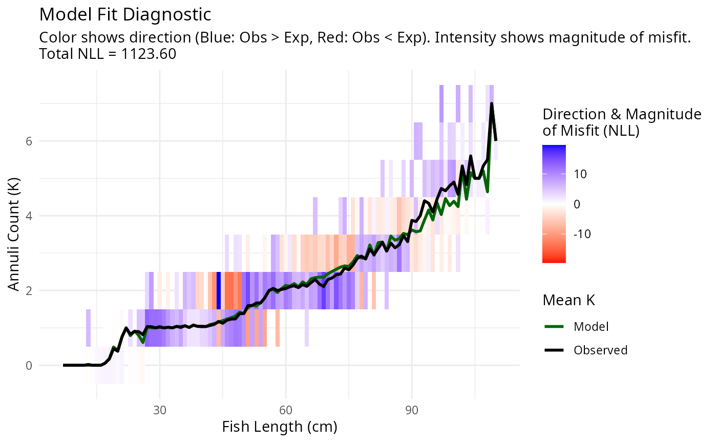

pars[parameter_names]

## $k
## [1] 0.1512644
## 
## $L_inf
## [1] 192.9295
## 
## $d
## [1] 1e-06
## 
## $m
## [1] 25
## 
## $annuli_min_age
## [1] 0

This leads to a more realistic time evolution of a yearly cohort:

u <- getNumberDensity(pars, l_max = 200, t_max = 15)
plotDensity2D(u)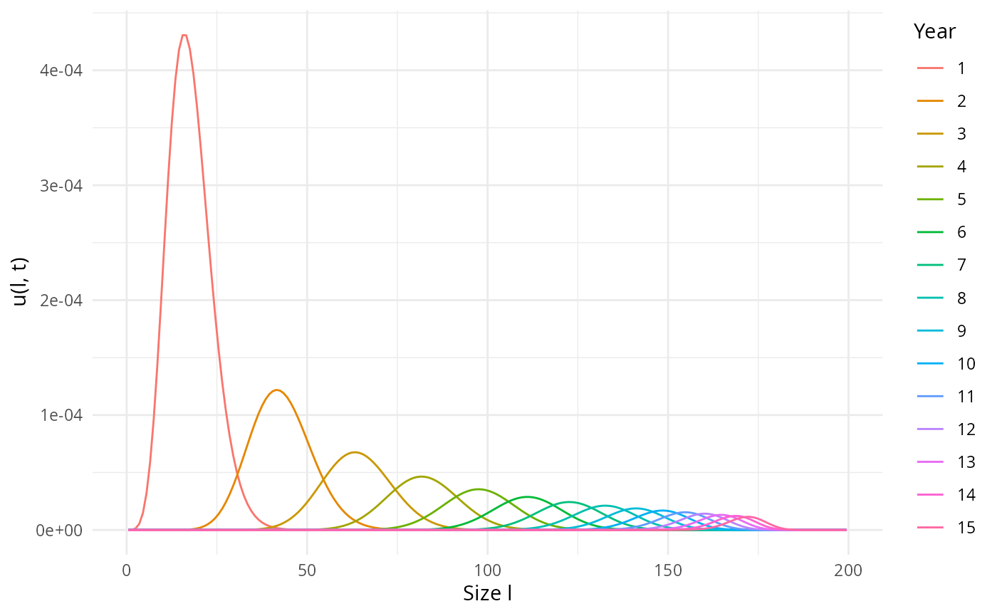

plotDensity3D(u, l_min = 20)

The solution including all yearly cohorts looks as follows:

u_periodic <- getPeriodicNumberDensity(pars, l_max = 200, t_max = 3)
plotDensity3D(u_periodic, l_min = 20)