Introduction
The trait-based size spectrum model can be derived as a simplification of the general model outline in the model description section. It is more complicated than a community model and the most significant difference between the two is that while the community model only resolves a single species, the trait-based model resolves many species. In a trait-based model the asymptotic size is considered to be the most important trait characterizing a species. All of the species-specific parameters, such as \(\beta\) and \(\sigma\), are the same for all species. Other model parameters are determined by the asymptotic size. For example, the weight at maturation, \(w_{m.i} = \eta w_{\infty.i}\), where \(\eta = 0.25\). The number of species is not important and does not affect the general dynamics of the model. The asymptotic sizes of the species are spread evenly over the size range of the community.
Setting up a trait-based model
To help set up a trait-based model, there is a wrapper function, set_trait_model(). Like the set_community_model() function described in the section on the community model, this function can take many arguments. Most of them have default values so you don’t need to worry about them for the moment. See the help page for more details.
The main parameters of interest are the number of the species in the model (no_sp) and the minimum and maximum asymptotic sizes (min_w_inf and max_w_inf respectively); the asymptotic sizes are spread evenly on a logarithmic scale between these values.
One of the key differences between the community type model and the trait-based model is that reproduction and egg production are considered. In the community model, recruitment is constant and there is no relationship between the abundance in the community and egg production. In the trait-based model, the egg production is modeled using a Beverton-Holt type function (the default in mizer, see the section on stock-recruitment relationships) where the recruitment flux \(R_i\) (numbers per time) approaches a maximum recruitment as the egg production increases. The maximum recruitment flux is calculated using equilibrium theory and a recruitment multiplier \(k_0\), which can be passed in as an argument (k0) to the set_trait_model() function. k0 has a default value of 50.
Here we set up the model to have 10 species, with asymptotic sizes ranging from 10 g to 100 kg. All the other parameters have default values.
The output reminds the user that \(\gamma\) was not specified, and so will be calculated using other parameters.
This function returns an object of type MizerParams, which holds all the model information, including species parameters.
## [1] "MizerParams"
## attr(,"package")
## [1] "mizer"
This object can therefore be interrogated in the same way as described in the section on the community model, either by inspecting the individual slots or by using the summary() function.
## An object of class "MizerParams"
## Community size spectrum:
##  minimum size:   0.001
##  maximum size:   110000
##  no. size bins:  100
## Background size spectrum:
##  minimum size:   1.03406e-10
##  maximum size:   110000
##  no. size bins:  186
## Species details:
##    species        w_inf        w_mat beta sigma
## 1        1     10.00000     2.500000  100   1.3
## 2        2     27.82559     6.956399  100   1.3
## 3        3     77.42637    19.356592  100   1.3
## 4        4    215.44347    53.860867  100   1.3
## 5        5    599.48425   149.871063  100   1.3
## 6        6   1668.10054   417.025134  100   1.3
## 7        7   4641.58883  1160.397208  100   1.3
## 8        8  12915.49665  3228.874163  100   1.3
## 9        9  35938.13664  8984.534160  100   1.3
## 10      10 100000.00000 25000.000000  100   1.3
## Fishing gear details:
##  Gear            Target species
##   knife_edge_gear         1 2 3 4 5 6 7 8 9 10
The summary shows us that now we have 10 species in the model, with asymptotic sizes ranging from
\(10\) to \(10^{5}\). The size at maturity (w_mat) is linearly related to the asymptotic size. Each species has the same preferred predator-prey mass ratio parameter values (beta and sigma, see the section on predator/prey mass ratio). There are \(100\) size bins in the community and \(186\) size bins including the plankton spectrum. Ignore the summary section on fishing gear for the moment. This is explained later.
Running the trait-based model
As with the community model described above, we can project the model through time using the project() method. Here we project the model for 75 time steps without any fishing (the effort argument is set to 0). We use the default initial population abundances given by the get_initial_n() function so there is no need to pass in any initial population values (see the section on setting the initial abundances).
This results in a MizerSim object which contains the abundances of the community and plankton spectra through time, as well as the original MizerParams object. As with the community model, we can get a quick overview of the results of the simulation by calling the generic plot() method:
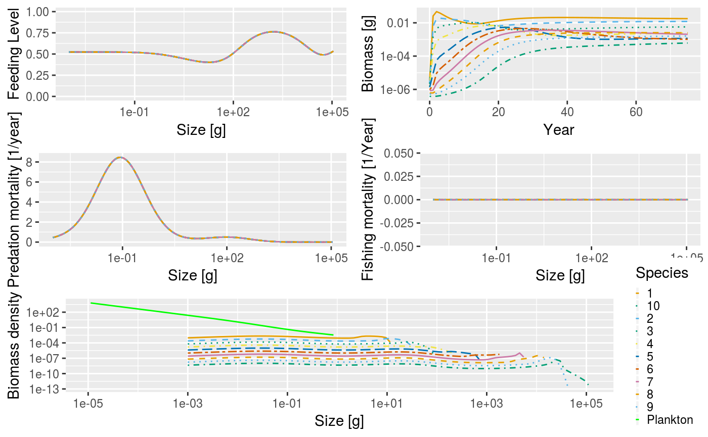
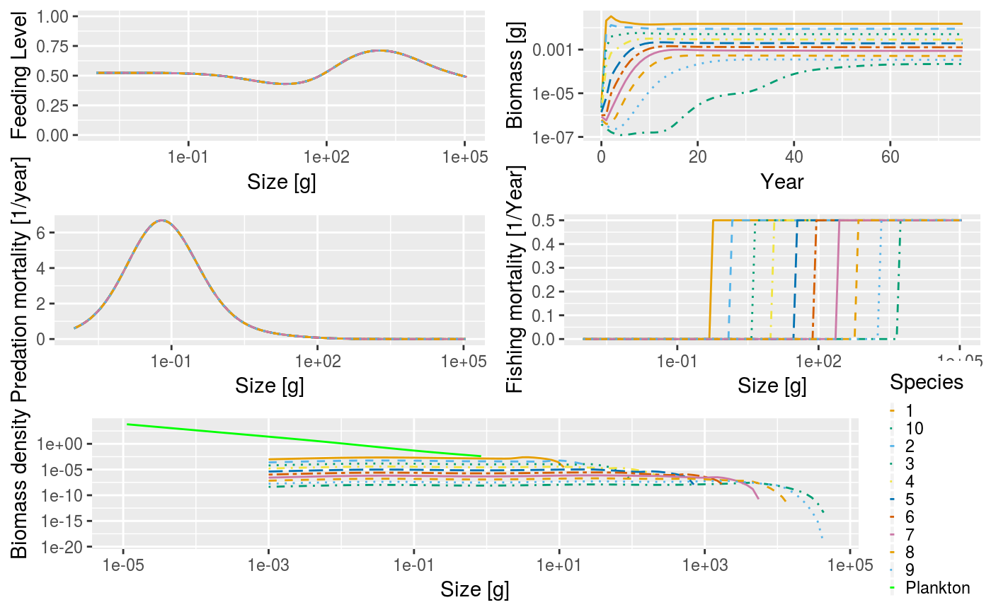
Example plot of the trait-based model with no fishing.
The summary plot has the same panels as the one generated by the community model, but here you can see that all the species in the community are plotted. The panels show the situation in the final time step of the simulation, apart from the biomass through time plot. As this is a trait-based model where all species fully interact with each other, the predation mortality (M2) and feeding level by size is the same for each species. The biomasses quickly settle down to equilibria. In this simulation we turned fishing off so the fishing mortality is 0. The size-spectra show the abundances at size to be evenly spaced by asymptotic size.
Example of a trophic cascade with the trait-based model
As with the community model, it is possible to use the trait-based model to simulate a trophic cascade. Again, we perform two simulations, one with fishing and one without. We therefore need to consider how fishing gears and selectivity have been set up by the set_trait_model() function.
The default fishing selectivity function is a knife-edge function, which only selects individuals larger than 1000 g. There is also only one fishing gear in operation, and this selects all of the species. You can see this if you call the summary() method on the params argument we set up above. At the bottom of the summary there is a section on Fishing gear details. You can see that there is only one gear, called `knife_edge_gear'' and that it selects species 1 to 10. To control the size at which individuals are selected there is aknife_edge_sizeargument to theset_trait_model()` function. This has a default value of 1000 g.
In mizer it is possible to include more than one fishing gear in the model and for different species to be caught by different gears. We will ignore this for now, but will explore it further below when we introduce an industrial fishery to the trait-based model.
To set up the trait-based model to have fishing we set up the MizerParams object in exactly the same way as we did before but here the knife_edge_size argument is explicitly passed in for clarity:
params_knife <- set_trait_model(no_sp = 10, min_w_inf = 10, max_w_inf = 1e5,
    knife_edge_size = 1000)
First we perform a simulation without fishing in the same way we did above by setting the effort argument to 0:
Now we simulate with fishing. Here, we use an effort of 0.75. As mentioned in the section on trophic cascades in the community model, the fishing mortality on a species is calculated as the product of effort, catchability and selectivity (see the section on fishing gears for more details). Selectivity ranges between 0 (not selected) and 1 (fully selected). The default value of catchability is 1. Therefore, in this simulation the fishing mortality of a fully selected individual is simply equal to the effort. This effort is constant throughout the duration of the simulation (however, this is does not necessarily have to be the case).
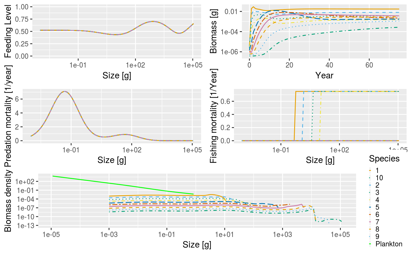
Again, we can plot the summary of the fished community using the default plot() function. The knife-edge selectivity at 1000 g can be clearly seen in the fishing mortality panel:
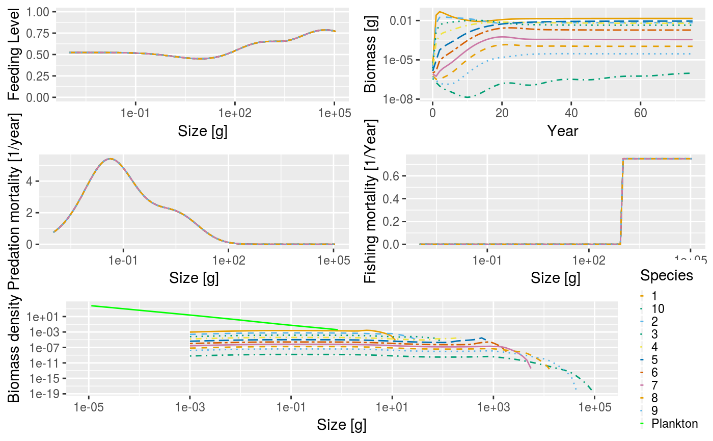
Summary plot for the trait-based model when fishing with knife-edge selectivity at size = 1000 g.
The trophic cascade can be explored by comparing the total abundances of all species at size when the community is fished and unfished. As mentioned above, the abundances are stored in the n slot of the MizerSim object. The n slot returns a three dimensional array with dimensions time x species x size. Here we have 76 time steps (75 from the simulation plus one which stores the initial population), 10 species and 100 sizes:
## [1] 76 10 100As with the community model, we are interested in the relative total abundances by size in the final time step so we want to pull out the 76th time step from the abundances and sum over the species. We can use the apply() function to help us:
We can then use these vectors to calculate the relative abundances:
Which can be plotted using the commands below:
plot(x=sim0@params@w, y=relative_abundance, log="xy", type="n", xlab = "Size (g)",
    ylab="Relative abundance", ylim = c(0.1,10))
lines(x=sim0@params@w, y=relative_abundance)
lines(x=c(min(sim0@params@w),max(sim0@params@w)), y=c(1,1),lty=2)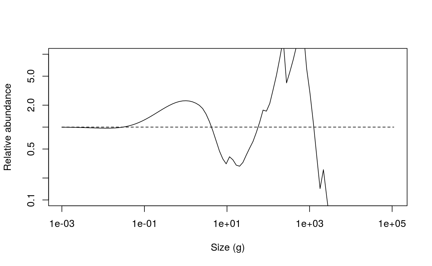
Relative abundances from the unfished (dashed line) and fished (solid line) trait based model.
The impact of fishing on species larger than 1000 g can be clearly seen. The fishing pressure lowers the abundance of large fish (\(> 1000\) g). This then relieves the predation pressure on their smaller prey (the preferred predator-prey size ratio is given by the \(\beta\) parameter, which is set to 100 by default), leading to an increase in their abundance. This in turn increases the predation mortality on their smaller prey, which reduces their abundance and so on.
This impact can also be seen by looking at the predation mortality by size. The predation mortalities are retrieved using the getM2() method for MizerSim objects. This returns a three dimensional array of predation mortalities by time x species x size (see the help page for getM2() for more details). As mentioned above, for the trait based model the predation mortality by size is the same for each species. Therefore we only look at the predation mortality of the first species.
The predation mortalities can then be plotted.
plot(x = sim0@params@w, y = m2_no_fishing, log="x", type="n", xlab = "Size (g)",
    ylab = "M2")
lines(x = sim0@params@w, y = m2_no_fishing, lty=2)
lines(x = sim0@params@w, y = m2_with_fishing)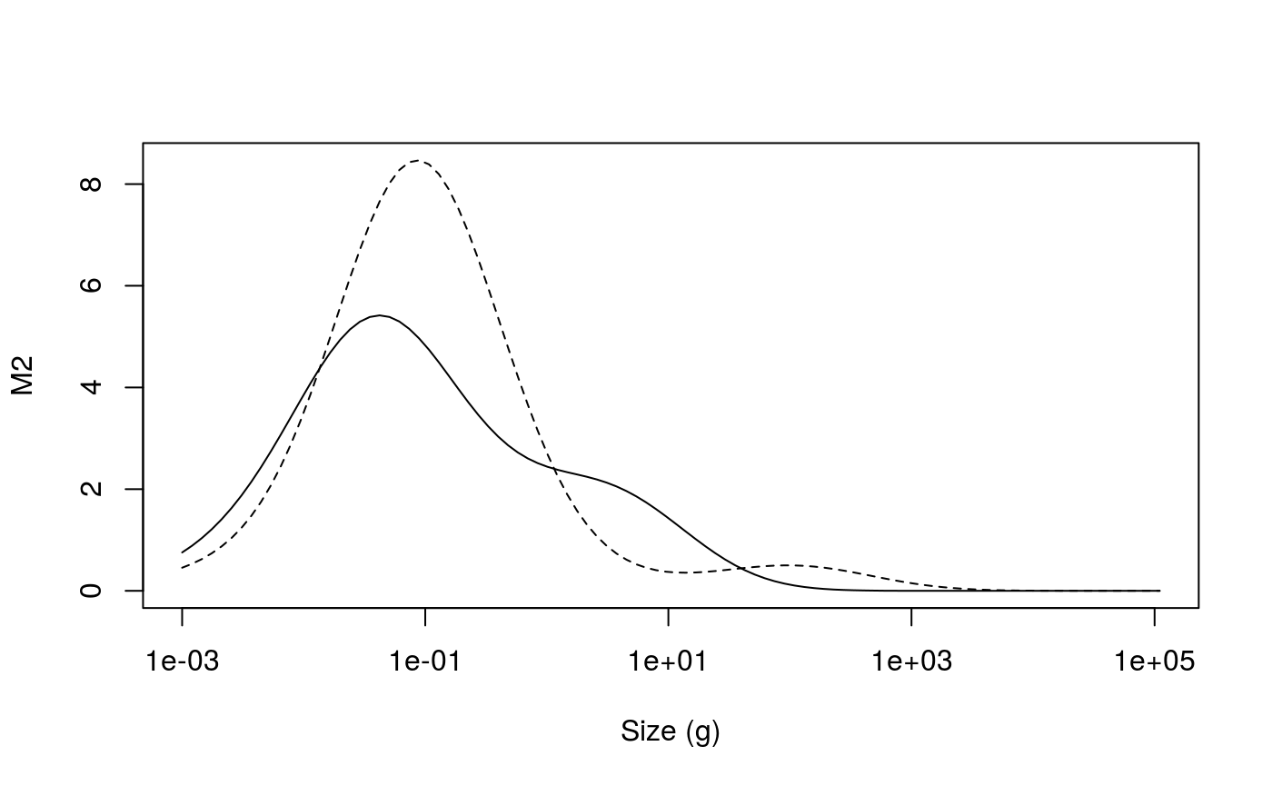
Predation mortalities from the unfished (dashed line) and fished (solid line) trait-based model.
Setting up an industrial fishing gear
In this section we only want to operate an industrial fishery. Industrial fishing targets the small zooplanktivorous species that are typically used for fishmeal production.
In the previous simulations we had only one fishing gear and it targeted all the species in the community. This gear had a knife-edge selectivity that only selected species larger than 1 kg. Here we expand the model to include multiple fishing gears. This requires us to look more closely at how fishing gears are handled in mizer. In mizer it is possible for a fishing gear to catch only a subset of the species in the model. This is useful because when running a simulation with project() you can specify the effort per gear and so you can turn gears on or off as you want. The shape of the selectivity function of each gear will be the same for all of the species it catches but the selectivity parameter values for each species may be different. For example, we can set up an industrial gear to catch only a subset of species. Each species it catches will be caught with knife-edge selectivity but they may have a different knife-edge positions.
Using the trait-based model wrapper function it is only possible to have a knife-edge selectivity. Each species in the model must be given the position of the knife edge and the name of the fishing gear. This is done using the knife_edge_size argument and the gear_names argument of the set_trait_model() function. In the previous examples, we passed in the knife_edge_size argument as a single value which was used for all the species. This effectively set up a single gear, that caught all species using the same selectivity pattern. The gear_names argument was not used. Now we are going to pass the knife_edge_size argument as a vector with the same length as the number of species in the model. The values in the vector will be the positions of the knife-edge for each species. We are also going to pass in a new argument, gear_names which is a vector of the names of the gears. The vector must have the same length as the number of species in the model.
We will set up the model to include two fishing gears: an industrial gear that only catches species with an asymptotic size less than or equal to 500g, and a second gear, ``other’’, that catches everything else. The position of the knife-edge for both gears will occur at 0.05 x the asymptotic size i.e. the selectivity parameters will be different for each species and will depend on the asymptotic size.
To start with we need to know what the asymptotic sizes of the species in the model are so we can determine the knife-edge positions for each species. As mentioned above, the set_trait_model() function spaces the asymptotic sizes equally on a logarithmic scale. This means we can calculate them by hand.
no_sp <- 10
min_w_inf <- 10
max_w_inf <- 1e5
w_inf <- 10^seq(from=log10(min_w_inf), to = log10(max_w_inf), length=no_sp)
We can then use these asymptotic sizes to set a vector of knife-edges that are 0.05 times the asymptotic size:
Now we want to assign each species to either the industrial or other gear, We want to create a vector of gear names. This vector must be the same length as the number of species in the model.
other_gears <- w_inf > 500
gear_names <- rep("Industrial", no_sp)
gear_names[other_gears] <- "Other"
Finally, we can create our MizerParams object by passing in the knife_edge_sizes and gear_names argument. All the other arguments are the same as before:
params_multi_gear <- set_trait_model(no_sp = no_sp, min_w_inf = min_w_inf,
    max_w_inf = max_w_inf, knife_edge_size = knife_edges, gear_names = gear_names)
To check what has just happened we can take a look inside the MizerParams object. There is a slot in the object called species_params. This is a data.frame that contains the life-history parameters of the species in the model (the results of running this command are not shown):
This data.frame is pretty interesting as it allows you to investigate the parameters for each species. For example, you can see that the predator-prey mass ratio parameters, beta and sigma, are indeed the same for each species. The columns of the species_params data.frame that we are interested in here are species (the name of the species, here just numerical identifiers), w_inf (the asymptotic size), sel_func (the name of the selectivity function for that species), knife_edge_size (the position of the knife-edge of the selectivity) and gear (the name of the fishing gear). You can see that two gears have been set up, Industrial and Other and that they catch different species depending on their asymptotic size.
Having created our MizerParams object with multiple gears, we can now turn our attention to running a projection with multiple gears. In our previous examples of calling project() we have specified the fishing effort with the effort argument using a single value. This fixes the fishing effort for all gears in the model, for all time steps. We can do this with our multi-gear parameter object:
By plotting this you can see that the fishing mortality for each species now has a different selectivity pattern, and that the position of the selectivity knife-edge is given by the asymptotic size of the species.
Summary plot for the trait-based model with multiple gears when all gears are operational.
For the industrial fishery we said that we only wanted species with an asymptotic size of 500 g or less to be fished. There are several ways of specifying the effort argument for project() . Above we specified a single value that was used for all gears, for all time steps. It is also possible to specify a separate effort for each gear that will be used for all time steps. To do this we pass in effort as a named vector. Here we set the effort for the Industrial gear to 0.75, and the effort of the Other gear to 0 (effectively turning it off).
Now you can see that the Industrial gear has been operating and that fishing mortality for species larger than 500 g is 0.
Summary plot for the trait-based model with multiple gears when only the industrial gear that fishes on species with asymptotic size of 500 g or less is operational.
The impact of industrial fishing
In the previous section we set up and ran a model in which an industrial fishery was operating that only selected smaller species. We can now answer the question: what is the impact of such a fishery? We can again compare abundances of the fished (sim_industrial1) and unfished (sim_industrial0) cases:
sim_industrial0 <- project(params_multi_gear, t_max = 75, effort = 0)
sim_industrial1 <- project(params_multi_gear, t_max = 75,
    effort = c(Industrial = 0.75, Other = 0))
total_abund0 <- apply(sim_industrial0@n[76,,],2,sum)
total_abund1 <- apply(sim_industrial1@n[76,,],2,sum)
relative_abundance <- total_abund1 / total_abund0
And plot the relative abundances:
plot(x=sim0@params@w, y=relative_abundance, log="xy", type="n", xlab = "Size (g)",
    ylab="Relative abundance", ylim = c(0.1,10))
lines(x=sim0@params@w, y=relative_abundance)
lines(x=c(min(sim0@params@w),max(sim0@params@w)), y=c(1,1),lty=2)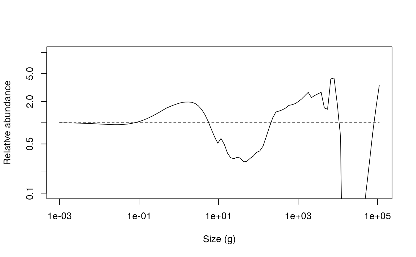
Relative abundances from the unfished (dashed line) and fished (solid line) trait based model with an industrial fishery that targets species with an asymptotic size of 500 g or less.
This shows another trophic cascade, although this time one driven by fishing the species at the midrange part of the spectrum, not the largest individuals as before. This trophic cascade acts in both directions. The cascade upwards is driven by the lack of food for predators leading to smaller realised maximum sizes. The cascade downwards has the same mechanism as fishing on large fish, a combination of predation mortality and food limitation.
The next section explains how to setup the more general multispecies model.