The General Mizer Size-spectrum Model
Edit this page. Source:vignettes/model_description.Rmd
model_description.RmdOn this page we will revisit the presentation of the mizer model given in chapter 3 of the main mizer vignette but taking care to separate the essential features of the model that are hard-coded and the various possible specialisations.
We will not go into detail of how this model is realised in code. Such detail will be provided in the developer guide. However some details are hidden on this page and you can see them by clicking on links like the following:Consumer size spectra
The model framework builds on two central assumption and a number of lesser standard assumption.
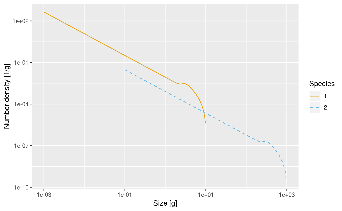
The first central assumption is that an individual can be characterized by its weight \(w\) and its species number \(i\) only. The aim of the model is to calculate the size spectrum \(N_i(w)\), which is the density of individuals of species \(i\) such that \(\int_w^{w+dw}N_i(w)dw\) is the number of individuals of species \(i\) in the size interval \([w,w+dw]\). In other word: the number of individuals in a size range is the area under the number density \(N_i(w)\).
Here is a plot of an example size spectrum for two species with \(N_i(w)\) on the vertical axis for \(i=1,2\) and \(w\) on the horizontal axis.
library(mizer)
params <- set_scaling_model(no_sp = 2, min_egg = 1e-3)
plotSpectra(params, plankton = FALSE, power = 0)
To represent this continuous size spectrum in the computer, the size variable \(w\) is discretized into a vector w of discrete weights, providing a grid of sizes spanning the range from the smallest egg size to the largest asymptotic size. These grid values divide the full size range into a finite number of size bins. The size bins should be chosen small enough to avoid the discretisation errors from becoming too big.
The weight grid is set up to be logarithmically spaced, so that w[j]=w[1]*exp(j*dx) for some fixed dx. This grid is set up automatically when creating a MizerParams object.
In the code the size spectrum is stored as an array such that n[i, a] holds the density \(N_i(w_a)\) at weights \(w_a=\)w[a], or, if time dependence is included, an array such that n[i, a, u] holds \(N_i(w_a,t_u)\).
Note that, contrary to what one might have expected, n[i, a] is not the number of individuals in a size bin but the density at a grid point. The number of individuals in the size bin between w[a] and w[a+1]=w[a]+dw[a] is only approximately given as n[i, a]*dw[a], where dw[a]= w[a+1]-w[a].
The time evolution of the size spectrum is described by the McKendrik-von Foerster equation, which is a continuity equation with loss:
\[\begin{equation} \label{eq:MvF} \frac{\partial N_i(w)}{\partial t} + \frac{\partial g_i(w) N_i(w)}{\partial w} = -\mu_i(w) N_i(w), \end{equation}\]
where individual growth \(g_i(w)\) and mortality \(\mu_i(w)\) will be described below.
This McKendrik-von Foerster equation is approximated in mizer by a finite-difference method (to be described in section …). This allows the project() method in mizer to project the size spectrum forwards in time: Given the spectrum at one time the project() method calculates it at a set of later times.
The McKendrik-von Foerster equation is supplemented by a boundary condition at the egg weight \(w_0\) where the flux of individuals (numbers per time) \(g_i(w_0)N_i(w_0)\) is determined by the rate \(R_i\) of production of offspring by mature individuals in the population: \[\begin{equation} g_i(w_0)N_i(w_0) = R_i. \end{equation}\]
In the code this boundary condition is actually implemented as an equation for the rate of change of the number of individuals in the smallest size bin: \[\begin{equation} \frac{dN_i(w_0)}{dt}=... \end{equation}\]
Resource size spectrum
Besides the fish spectrum there is also a resource spectrum \(N_R(w)\), representing for example the phytoplankton. This spectrum starts at a smaller size than the fish spectrum, in order to provide food also for the smallest individuals (larvae) of the fish spectrum.
By default the time evolution of the resource spectrum is described by a semi-chemostat equation: \[\begin{equation}
\label{eq:nb}
\frac{\partial N_R(w,t)}{\partial t}
= r_p(w) \Big[ c_p (w) - N_R(w,t) \Big] - \mu_p(w) N_R(w,t).
\end{equation}\] Here \(r_p(w)\) is the plankton regeneration rate and \(c_p(w)\) is the carrying capacity in the absence of predation. These parameters are changed with changePlankton(). By default mizer assumes allometric forms \[r_p(w)= r_p\, w^{n-1}.\] \[c_p(w)=\kappa\, w^{-\lambda}.\] It is also possible to implement other plankton dynamics, as described in the help page for changePlankton(). The death \(\mu_p(w)\) is described in the subsection Plankton mortality.
Because the plankton spectrum spans a different range of sizes these sizes are discretized into a different vector of weights w_full. The last entries of w_full have to coincide with the entries of w. The resource spectrum is then stored in a vector n_pp such that n_pp[c] =\(N_R(\)w_full[c]\()\).
The plankton regeneration rate is stored as a vector params@rr_pp[c]\(=r_p(\)w_full[c]\()\), and the carrying capacity is stored as a vector params@cc_pp[c]\(=c_p(\)w_full[c]\()\).
Predator-prey encounter rate
The rate at which a predator of species \(i\) and weight \(w\) encounters food (mass per time) is determined by summing over all prey species and the resource spectrum and integrating over all prey sizes \(w_p\), weighted by the selectivity factors: \[\begin{equation}
\label{eq:1}
E_{i}(w) = \gamma_i(w) \int \left(\sum_{j} \theta_{ij} N_j(w_p) +
\theta_{ip} N_R(w_p) + \right)
\phi_i(w,w_p) w_p \, dw_p.
\end{equation}\] The overall prefactor \(\gamma_i(w)\) sets the predation power of the predator. It could be interpreted as a search volume. It is set by changeSearchVolume(). By default it is assumed to scale allometrically as \(\gamma_i(w) = \gamma_i\, w^q.\)
The \(\theta\) matrix sets the interaction strength between predators and the various prey species and plankton. It is changed with changeInteraction().
The size selectivity is encoded in the predation kernel \(\phi_i(w,w_p)\). This is changed with changePredKernel().
An important simplification occurs when the predation kernel \(\phi_i(w,w_p)\) depends on the size of the prey only through the predator/prey size ratio \(w_p/w\), \[\phi_i(w, w_p)=\tilde{\phi}_i(w/w_p).\] This is assumed by default but can be overruled. The default for the predation kernel is the truncated log-normal function \[ \label{eq:4} \tilde{\phi}_i(x) = \begin{cases} \exp \left[ \dfrac{-(\ln(x / \beta_i))^2}{2\sigma_i^2} \right] &\text{ if }x\in\left[0,\beta_i\exp(3\sigma_i)\right]\\ 0&\text{ otherwise,} \end{cases} \] where \(\beta_i\) is the preferred predator-prey mass ratio and \(\sigma_i\) sets the width of the predation kernel.
The integral in the expression for the encounter rate is approximated by a Riemann sum over all weight brackets: \[ {\tt encounter}[i,a] = {\tt search\_vol}[i,a]\sum_{k} \left( n_{pp}[k] + \sum_{j} \theta[i,j] n[j,k] \right) \phi_i\left(w[a],w[k]\right) w[k]\, dw[k]. \] In the case of a predation kernel that depends on \(w/w_p\) only, this becomes a convolution sum and can be evaluated efficiently via fast Fourier transform.
Consumption
The encountered food is consumed subjected to a standard Holling functional response type II to represent satiation. This determines the feeding level \(f_i(w)\), which is a dimensionless number between 0 (no food) and 1 (fully satiated) so that \(1-f_i(w)\) is the proportion of the encountered food that is consumed. The feeding level is given by
\[\begin{equation} \label{eq:f} f_i(w) = \frac{E_{i}(w)}{E_{e.i}(w) + h_i(w)}, \end{equation}\]
where \(h_i(w)\) is the maximum consumption rate. This is changed with changeIntakeMax(). By default mizer assumes an allometric form \(h_i(w) = h_i\, w^n.\)
The rate at which food is consumed is then \[\begin{equation} (1-f_i(w))E_{i}(w)=f_i(w)\, h_i(w). \end{equation}\]
Metabolic losses
Some of the consumed food is used to fuel the needs for metabolism and activity and movement, at a rate \({\tt metab}_i(w)\). By default this is made up out of standard metabolism, scaling with exponent \(p\), and loss due to activity and movement, scaling with exponent \(1\): \[{\tt metab}_i(w) = k_{s.i}\,w^p + k_i\,w.\] See the help page for changeMetab().
The remaining rate, if any, is assimilated with an efficiency \(\alpha_i\) and is then available for growth and reproduction. So the rate at which energy becomes available for growth and reproduction is \[\begin{equation} \label{eq:Er} E_{r.i}(w) = \max(0, \alpha_i f_i(w)\, h_i(w) - {\tt metab}_i(w)) \end{equation}\]
Investment into reproduction
A proportion \(\psi_i(w)\) of the energy available for growth and reproduction is used for reproduction. This proportion should change from zero below the weight \(w_{m.i}\) of maturation to one at the asymptotic weight \(w_{\infty.i}\), where all available energy is used for reproduction. This function is changed with changeReproduction(). Mizer provides a default form for the function which you can however overrule.
The total production rate of egg production \(R_{p.i}\) (numbers per year) is found by integrating the contribution from all individuals of species \(i\): \[\begin{equation} \label{eq:Rp} R_{p.i} = \frac{\epsilon}{2 w_0} \int N_i(w) E_{r.i}(w) \psi_i(w) \, dw, \end{equation}\] where the individual contribution is obtained by multiplying the rate at which the individual allocates energy to reproduction by an efficiency factor \(\epsilon\) and then dividing by the egg weight \(w_0\) to convert the energy into number of eggs. The result is multiplied by a factor \(1/2\) to take into account that only females reproduce.
Recruitment
In mizer, density dependence is modelled as a compensation on the egg production. This can be considered as the stock-recruitment relationship (SRR). The default functional form is such that the recruitment flux \(R_i\) (numbers per time) approaches a maximum recruitment as the egg production increases, modelled mathematically analogous to the Holling type II function response as a Beverton-Holt type of SRR:
\[\begin{equation} \label{eq:R} R_i = R_{\max.i} \frac{R_{p.i}}{R_{p.i} + R_{\max.i}}, \end{equation}\] where \(R_{\max.i}\) is the maximum recruitment flux of each trait class (Figure~).
The Beverton-Holt type of SRR is not the only density dependence model that mizer can use. Users are able to write their own model so it is possible to set a range of SRRs, e.g. fixed recruitment (as used in the community-type model) or hockey-stick.
Growth
What is left over after metabolism and reproduction is taken into account is invested in somatic growth. Thus the growth rate is \[\begin{equation} \label{eq:growth} g_i(w) = E_{r.i}(w)\left(1-\psi_i(w)\right). \end{equation}\]
When food supply does not cover the requirements of metabolism and activity, growth and reproduction stops, i.e. there is no negative growth. The individual should then be subjected to a starvation mortality, but starvation mortality is not implemented in mizer at the moment.
Mortality
The mortality rate of an individual \(\mu_i(w)\) has three sources: predation mortality \(\mu_{p.i}(w)\), background mortality \(\mu_{b.i}(w)\) and fishing mortality \(\mu_{f.i}(w)\).
Predation mortality is calculated such that all that is eaten translates into corresponding predation mortalities on the ingested prey individuals. Recalling that \(1-f_j(w)\) is the proportion of the food encountered by a predator of species \(j\) and weight \(w\) that is actually consumed, the rate at which all predators of species \(j\) consume prey of size \(w_p\) is \[\begin{equation} \label{eq:pred_rated} {\tt pred\_rate}_j(w_p) = \int \phi_j(w,w_p) (1-f_j(w)) \gamma_j(w) N_j(w) \, dw. \end{equation}\]
The integral is approximated by a Riemann sum over all fish weight brackets. \[ {\tt pred\_rate}[j,c] = \sum_{a} {\tt pred_kernel}[j,a,c]\,(1-{\tt feeding_level}[j,a])\, \gamma[j,a]\,n[j,a]\,dw[a]. \]
The mortality rate due to predation is then obtained as \[\begin{equation} \label{eq:mup} \mu_{p.i}(w_p) = \sum_j {\tt pred\_rate}_j(w_p)\, \theta_{ji}. \end{equation}\]
Background mortality \(\mu_{b .i}(w)\) is independent of the abundances and is changed with changeBMort(). By default mizer assumes an allometric form \[\mu_{b.i}(w) = \mu_b w_{\infty.i}^{1-n},\] where \(w_{\infty.i}\) is the asymptotic size of species \(i\).
Fishing mortality \(\mu_{f.i}(w)\) will be discussed in section Fishing.
The total mortality rate is \[\mu_i(w)=\mu_{p.i}(w)+\mu_{b.i}(w)+\mu_{f.i}(w)\]
Plankton Mortality
The predation mortality rate on plankton is given by a similar expression as the predation mortality on fish: \[\begin{equation} \label{eq:mupp} \mu_{p}(w_p) = \sum_j {\tt pred\_rate}_j(w_p)\, \theta_{jp}. \end{equation}\] This is the only mortality on plankton currently implemented in mizer.