Exploring the Simulation Results
Edit this page. Source:vignettes/exploring_the_simulation_results.Rmd
exploring_the_simulation_results.RmdIntroduction
In the sections on the multispecies model and on running a simulation we saw how to set up a model and project it forward through time under our desired fishing scenario. The result of running a projection is an object of class MizerSim. What do we then do? How can we explore the results of the simulation? In this section we introduce a range of summaries, plots and indicators that can be easily produced using functions included in mizer.
We will use the same MizerSim object for these examples:
Directly accessing the slots of MizerSim objects
We have seen in previous sections that a MizerSim object is made up of various slots that contain the original parameters (species_params), the population abundances (n), the abundance of the plankton spectrum (n_pp), possibly the biomasses of unstructured resources (B), and the fishing effort (effort).
The projected species abundances at size through time can be seen in the n slot. This is a three-dimensional array (time x species x size). Consequently, this array can get very big so inspecting it can be difficult. In the example we have just run, the time dimension of the n slot has 10 rows (one for the initial population and then one for each of the saved time steps). There are also 12 species each with 100 sizes. We can check this by running the dim() function and looking at the dimensions of the n array:
## [1] 10 12 100To pull out the abundances of a particular species through time at size you can subset the array. For example to look at Cod through time you can use:
This returns a two-dimensional array: time x size, containing the cod abundances. The time dimension depends on the value of the argument t_save when project() was run. You can see that even though we specified dt to be 0.1 when we called project(), the t_save = 1 argument has meant that the output is only saved every uear.
The n_pp slot can be accessed in the same way.
Summary methods for MizerSim objects
As well as the summary() methods that are available for both MizerParams and MizerSim objects, there are other useful summary methods to pull information out of a MizerSim object. A description of the different summary methods available is given in the summary methods help page.
All of these methods have help files to explain how they are used. (It is also possible to use most of these methods with a MizerParams object if you also supply the population abundance as an argument. This can be useful for exploring how changes in parameter value or abundance can affect summary statistics and indicators. We won’t explore this here but you can see their help files for more details.)
The methods getBiomass() and getN() have additional arguments that allow the user to set the size range over which to calculate the summary statistic. This is done by passing in a combination of the arguments min_l, min_w, max_l and max_w for the minimum and maximum length or weight.
If min_l is specified there is no need to specify min_w and so on. However, if a length is specified (minimum or maximum) then it is necessary for the species parameter data.frame (see the species parameters section) to include the parameters a and b for length-weight conversion. It is possible to mix length and weight constraints, e.g. by supplying a minimum weight and a maximum length. The default values are the minimum and maximum weights of the spectrum, i.e. the full range of the size spectrum is used.
Examples of using the summary methods
Here we show a simple demonstration of using a summary method using the sim object we created earlier. Here, we use getSSB() to calculate the SSB of each species through time (note the use of the head() function to only display the first few rows).
## [1] 10 12## sp
## time Sprat Sandeel N.pout Herring Dab
## 1 36029938 5.472992e+07 35571252 2.990330e+07 38479325
## 2 177009866 2.430069e+10 4377323145 1.965994e+08 659129339
## 3 11097299999 4.804739e+11 265729744953 2.428886e+10 13228260702
## 4 87560006143 1.083163e+12 379299271628 1.978630e+11 39036109165
## 5 351265713190 1.468707e+12 374498905229 6.689569e+11 55641581646
## 6 448897618861 1.489816e+12 273063416658 1.169533e+12 52156542433
## sp
## time Whiting Sole Gurnard Plaice Haddock Cod
## 1 29928416 29191048 34484711 25984507 25961161 20055185
## 2 14091030 13739444 16293490 10092378 15575659 7626973
## 3 563996697 147257604 261168563 4561258 1177016873 3715821
## 4 5050394382 3367749582 1852502768 4207003 15549083633 28086231
## 5 38424324147 19220173163 3069832259 45016372 43153790789 3948533926
## 6 117652804933 46520219197 3030919441 211853466 80182360951 53439339893
## sp
## time Saithe
## 1 21521377
## 2 8169171
## 3 3579942
## 4 2716818
## 5 4416665
## 6 33596280As mentioned above, we can specify the size range for the getBiomass() and getN() methods. For example, here we calculate the total biomass of each species but only include individuals that are larger than 10 g and smaller than 1000 g.
##     sp
## time        Sprat      Sandeel       N.pout      Herring          Dab
##    1     49041758 5.654440e+07     51582276 4.931529e+07     51017971
##    2    490779088 3.721918e+09  25999573964 1.952166e+10   5240583260
##    3  25783850174 2.377446e+11 581015555516 3.086905e+11  55404975864
##    4 186375227047 9.017899e+11 549591259535 1.366428e+12 100965688745
##    5 662355802154 1.403032e+12 526356288182 3.311079e+12 113391969285
##    6 718764900806 1.478552e+12 369262268192 3.608094e+12  90172174232
##     sp
## time      Whiting         Sole     Gurnard     Plaice      Haddock
##    1     34694997     41533451    46484086   12489697     10470857
##    2    500106124    735729465   303592284    8919217   5152082008
##    3   6737301137  19574964756  7192092253  188000256  46783953949
##    4  30614329729  76124227629 11590109862 1039980660 116331943624
##    5 179933503465 191006534379 13979237136 2231031403 275529691865
##    6 294995192308 313047042276 16680463810 2867229959 439216232650
##     sp
## time          Cod     Saithe
##    1 6.853965e+05    1801217
##    2 1.758179e+06    2850771
##    3 4.463547e+07    5245032
##    4 3.078709e+09   68143228
##    5 3.809203e+10  633270381
##    6 1.062645e+11 2375934419
Methods for calculating indicators
Methods are available to calculate a range of indicators from a MizerSim object after a projection. A description of the different indicator methods available is given in the summary methods help page. You can read the help pages for each of the methods for full instructions on how to use them, along with examples.
With all of the methods in the table it is possible to specify the size range of the community to be used in the calculation (e.g. to exclude very small or very large individuals) so that the calculated metrics can be compared to empirical data. This is used in the same way that we saw with the method getBiomass() in the section on summary methods for MizerSim objects. It is also possible to specify which species to include in the calculation. See the help files for more details.
Examples of calculating indicators
For these examples we use the sim object we created earlier.
The slope of the community can be calculated using the getCommunitySlope() method. Initially we include all species and all sizes in the calculation (only the first five rows are shown):
##        slope intercept        r2
## 1 -0.4970061  14.32058 0.7198141
## 2 -1.3011668  21.06361 0.8257857
## 3 -1.4159126  22.74646 0.7787319
## 4 -1.3675689  23.36632 0.7380701
## 5 -1.1725300  23.93529 0.6890267
## 6 -1.0015954  24.25681 0.6612782
This gives the slope, intercept and \(R^2\) value through time (see the help file for getCommunitySlope for more details).
We can include only the species we want with the species argument. Below we only include demersal species. We also restrict the size range of the community that is used in the calculation to between 10 g and 5 kg. The species is a character vector of the names of the species that we want to include in the calculation.
dem_species <- c("Dab", "Whiting", "Sole", "Gurnard", "Plaice", "Haddock",
    "Cod", "Saithe")
slope <- getCommunitySlope(sim, min_w = 10, max_w = 5000,
    species = dem_species)
head(slope)
## slope intercept r2
## 1 -0.6612095 15.26977 0.6978218
## 2 -2.3162432 25.92822 0.9734768
## 3 -3.0278183 31.57988 0.9615633
## 4 -2.5932457 31.20778 0.9255678
## 5 -1.6901969 28.59093 0.9529838
## 6 -1.1481856 26.69365 0.9338925Plotting the results
R is very powerful when it comes to exploring data through plots. A useful package for plotting is ggplot2. ggplot2 uses data.frames for input data. Many of the summary methods and slots of the mizer classes are arrays or matrices. Fortunately it is straightforward to turn arrays and matrices into data.frames using the command melt which is in the reshape2 package. Although mizer does include some dedicated plots, it is definitely worth your time getting to grips with these ggplot2 and other plotting packages. This will make it possible for you to make your own plots.
Included in mizer are several dedicated plots that use MizerSim objects as inputs (see the plots help page.). As well as displaying the plots, these methods all return objects of type ggplot from the ggplot2 package meaning that they can be further modified by the user (e.g. by changing the plotting theme). See the help page of the individual plot methods for more details. The generic plot() method has also been overloaded for MizerSim objects. This produces several plots in the same window to provide a snapshot of the results of the simulation.
Some of the plots plot values by size (for example plotFeedingLevel() and plotSpectra()). For these plots, the default is to use the data at the final time step of the projection. With these plotting methods, it is also possible to specify a different time step or a time range to average the values over before plotting.
Plotting examples
Using the plotting methods is straightforward. For example, to plot the total biomass of each species against time you use the plotBiomass() method:
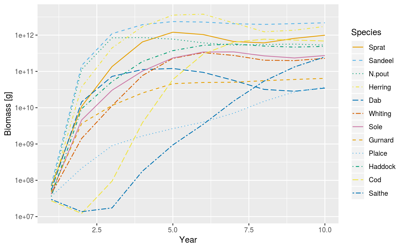
An example of using the plotBiomass() method.
As mentioned above, some of the plot methods plot values against size at a point in time (or averaged over a time period). For these plots it is possible to specify the time step to plot, or the time period to average the values over. The default is to use the final time step. Here we plot the abundance spectra (biomass), averaged over time = 5 to 10:
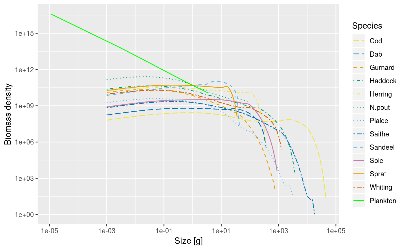
An example of using the plotSpectra() method, plotting values averaged over the period t = 5 to 10.
As mentioned above, and as we have seen several times in this vignette, the generic plot() method has also been overloaded. This produces 5 plots in the same window (plotFeedingLevel(), plotBiomass(), plotM2(), plotFMort() and plotSpectra()). It is possible to pass in the same arguments that these individual plots use, e.g. arguments to change the time period over which the data is averaged.
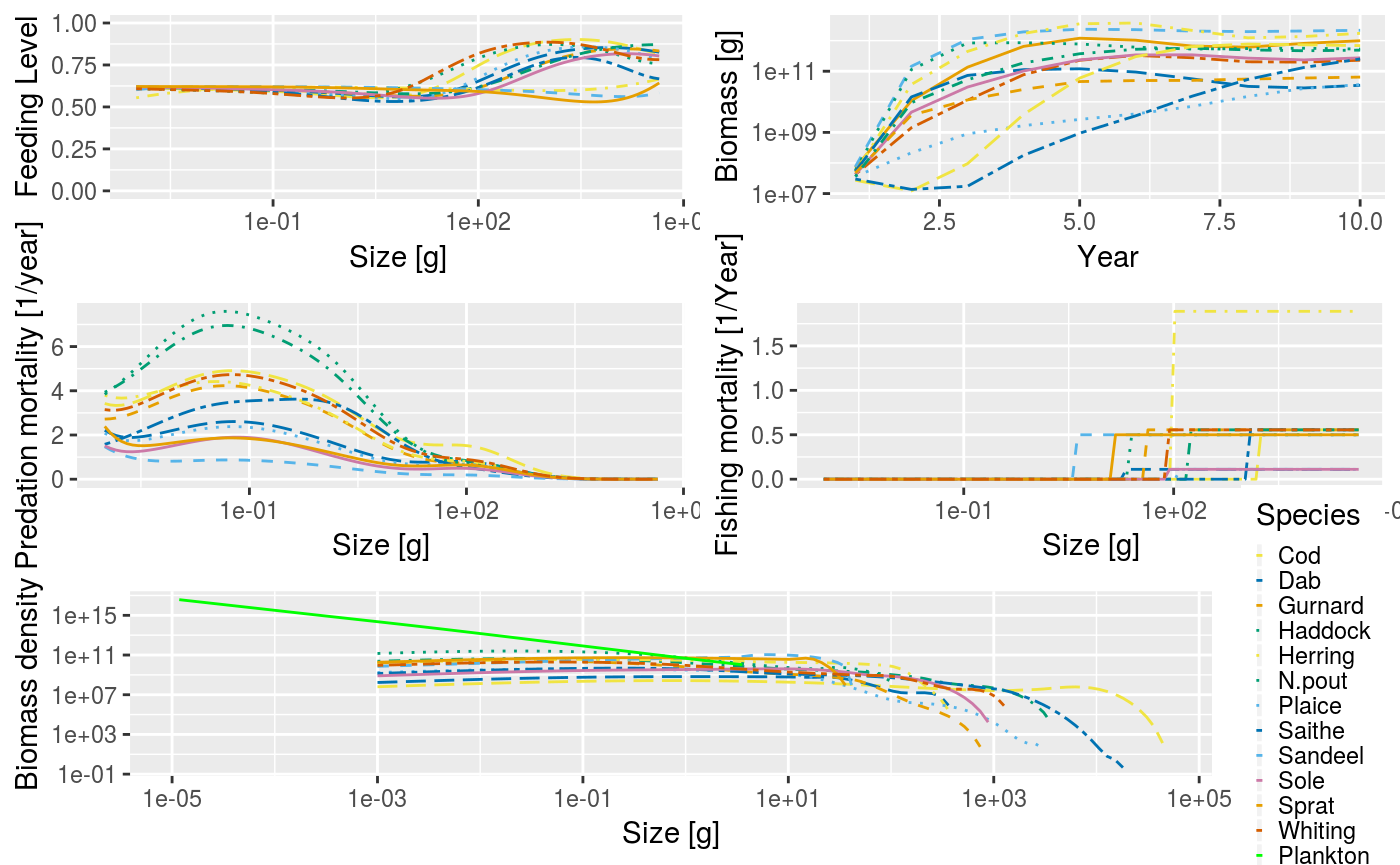
Example output from using the summary plot() method.
The next section describes how to use what we have used to model the North Sea.